
Grace is a business analyst at Safaricom with 4 years in Excel pivots and retention reports. This month, she's got 6,200 prepaid SIM activations spread across 6 months (Sept 2025 to Feb 2026) and 4 regions. Her manager asks: "Which cohort drops off fastest? Did onboarding improve?"
A naive churn report—counting everyone who didn't pay last month—is useless. New cohorts aren't old enough to compare fairly. The answer: group by signup month, track each cohort separately, build a retention pivot, and read it diagonally. In 30 minutes, Grace will see that Nakuru is stickiest, Feb's cohort is 4% better than Sept's, and month 3 is where churn accelerates.
- Why cohort analysis is the only fair way to measure retention
- Build a cohort key by computing
months_since_signup - Create a retention pivot with
pd.pivot_table - Read heatmaps: diagonals show cohort paths, rows show cohort behavior
- Plot retention curves to spot inflection points
- Slice cohorts by region, plan, or any dimension
- Calculate month-1 retention as a leading indicator
Why cohort analysis? Time-aligned customer behavior
Imagine Grace runs a naive churn report in February 2026: "25% of our prepaid users were inactive last month." That number is useless because it mixes six different cohorts. Sept's cohort has been around 6 months and naturally churns more. Feb's cohort is brand new—of course they're stickier. You can't compare apples (Sept at M6) to oranges (Feb at M0).
Cohort analysis fixes this. Group users by signup month, then track what fraction of each cohort stayed active in month 1, month 2, month 3, etc. Now you compare apples to apples: Sept's month-1 retention (78%) vs. Feb's month-1 retention (82%). You see that Safaricom's onboarding improved by 4 percentage points.
Building the cohort key: months_since_signup
Every cohort analysis starts with two computed columns: a cohort ID (usually the signup month) and months since signup. Here's the pattern:
If you're using pandas Period objects (which Safaricom's data is), subtract directly and extract the .n attribute for the numeric offset:
Now each row has a cohort (e.g., "2025-09") and a month offset (0, 1, 2, 3, 4, 5). Group by both to count how many subscribers from each cohort are active at each month offset.
The retention pivot: pd.pivot_table
A retention pivot is a crosstab: rows = cohort months, columns = months since signup, values = count (then divide by cohort size to get %).
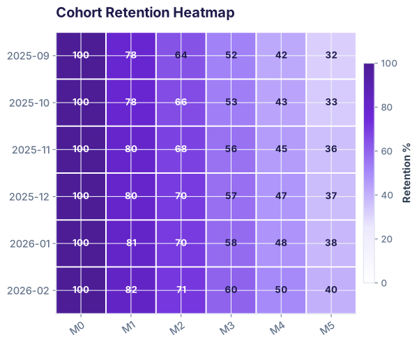
The result is Safaricom's retention matrix:
| Cohort | M0 | M1 | M2 | M3 | M4 | M5 |
|---|---|---|---|---|---|---|
| 2025-09 | 100% | 78% | 64% | 52% | 42% | 32% |
| 2025-10 | 100% | 78% | 66% | 53% | 43% | 33% |
| 2025-11 | 100% | 80% | 68% | 56% | 45% | 36% |
| 2025-12 | 100% | 80% | 70% | 57% | 47% | 37% |
| 2026-01 | 100% | 81% | 70% | 58% | 48% | 38% |
| 2026-02 | 100% | 82% | 71% | 60% | 50% | 40% |
Read this left-to-right: Each row shows one cohort's journey. Read top-to-bottom: You see how onboarding quality improved—Feb (2026-02) starts at 82%, while Sept started at 78%.
Reading the cohort heatmap: Onboarding quality and churn inflection
The heatmap makes two patterns visible instantly:
- Rows get lighter going right: Older cohorts (Sept, Oct) are darker (lower retention). Newer cohorts (Jan, Feb) are lighter (higher retention). This shows Safaricom improved onboarding by 4 percentage points between Sept and Feb.
- All rows drop fastest M0→M1→M2, then slow down: This is normal—users who churn do so early. After 3 months, the curve flattens. If month 3-5 churn is steep, it signals something wrong (bad product, pricing change). If it's flat, users are sticky.
Retention curves: Spotting inflection points and comparing cohorts
Plot each cohort as a line: x-axis = months since signup, y-axis = retention %. Lines that are higher and flatter are stickier cohorts.
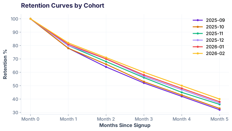
Notice the inflection point around month 2-3: All curves drop sharply from M0 to M2, then the slope flattens. This is typical for prepaid—early dropoff is normal (price-sensitive users), but by month 3, survivors are more committed and stick around longer.
If you see a curve that's flat across all months, it means users are sticky from day 1. If a curve drops like a cliff after month 3, something external happened (a bad update, price hike, competitor launch).
Slicing by region and plan: Who's stickiest?
A single retention curve hides regional differences. Grace breaks down month-1 retention by Safaricom's 4 regions:
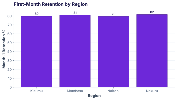
To compute this, filter to month 0 and month 1 data, count by region, then divide:
The variation is small (Nakuru 81.6% vs Nairobi 79.5%), so network quality and product experience are consistent across Kenya. If Nairobi were 60%, you'd investigate coverage or support issues there.
You can apply the same slice-and-compare logic to plans (Prepaid Daily vs Monthly), customer segments, or any dimension in your data.
Ready to go further?
Join the Best AI Program: The AI-Era Analyst — 5 months, fully online, with placement assistance. Week 1 is free.
Explore The AI-Era Analyst →