
💼
Real-world scenario
Arjun (Hyderabad, fintech): Summarizing a loan portfolio in one page

Arjun works nights as a data analyst at a consumer loan fintech in Hyderabad. Tomorrow he'll present his first credit-committee meeting — a room of risk officers and executives. He has 150 loan records and 15 minutes to build one-pager summary slides.

Instead of manually scanning CSV rows, he runs df.describe(). In five seconds, he sees the mean loan amount, its spread, outliers, and distribution shape. The numbers go straight onto his slide. Same stats work for any loan portfolio — Mumbai, São Paulo, Lagos — the shape of lending data is universal.

150
Loans in portfolio
₹102k
Mean amount
1.8
Skewness
What you'll learn
  • Run .describe() for instant summaries
  • Understand mean vs median and when each matters
  • Measure spread with std, variance, IQR, and range
  • Spot skewed & kurtotic distributions
  • Describe categorical columns with .describe(include='object')
  • Calculate custom percentiles with .quantile()
  • Unlock groupby summaries for next lesson

The one-shot summary: df.describe()

When you have a DataFrame with numerical columns, df.describe() runs eight statistics at once and displays them in a styled table.

📁
Sample loan data included
Download loan_portfolio.csv to follow along (150 loans, skewed distribution).
Stat amount_inr interest_rate tenure_months applicant_age credit_score
count 130.0 150.0 150.0 150.0 150.0
mean 116,469 12.7 54.5 37.8 718.0
std 89,803 1.4 19.2 9.7 64.1
min 28,000 9.8 24.0 23.0 580.0
25% 59,250 11.7 42.0 29.0 670.0
50% (median) 77,500 12.7 54.0 36.0 720.0
75% 153,750 13.8 66.0 45.0 770.0
max 420,000 15.5 102.0 60.0 825.0
Load and summarize
What this shows: count = non-missing rows (150 loans, but amount_inr has 130 — 20 missing). mean = average; loan amounts average ₹116k. std = scatter around the mean; loans vary by ₹90k on average — high, indicating skew. min/max = extreme values; smallest loan is ₹28k, largest is ₹420k. 25%, 50%, 75% = quartiles that split data into four equal groups; notice the median (₹77.5k) is well below the mean — a classic right-skew signal.

Mean vs median: the skew tells the story

Both measure "center" but behave differently when data is skewed. The histogram below shows loan amounts with mean (blue), median (amber), and mode (green) marked.
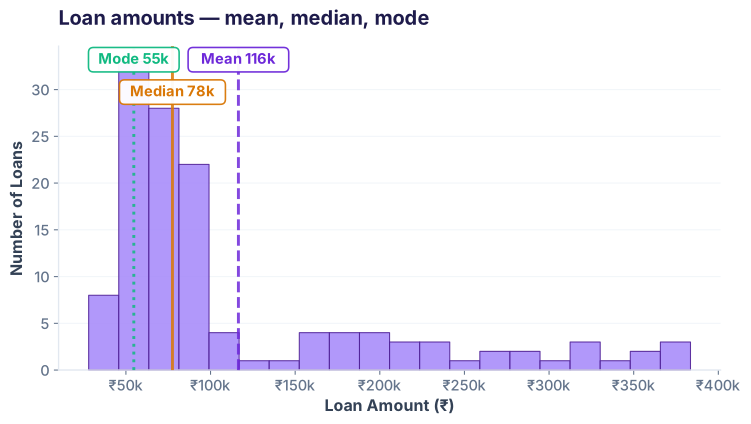
Loan amount distribution: mean, median, and mode
Histogram of loan amounts with mean (purple dashed), median (amber solid), and mode (green dotted) lines. Mean at ₹116k sits well to the right of the median at ₹78k.
Compare the three
What this shows: The mean (₹116k) sits well to the right of the median (₹78k) — a classic right-skewed distribution. The tallest bin (mode ≈ ₹55k) marks where most borrowers cluster; a long tail of larger loans drags the mean up. When mean ≫ median, ask: are those whales legitimate (enterprises, wealthy borrowers) or data-entry errors?

Measures of spread: std, variance, IQR, range

Standard deviation (std) tells you how scattered data is around the mean. Variance is std squared. IQR (interquartile range) is robust to outliers. Range is just max − min.
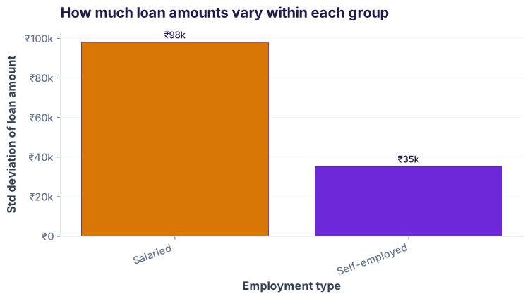
Standard deviation of loan amounts by employment type
Bar chart comparing standard deviation of loan amounts across employment types. Salaried borrowers show much higher variability than Self-employed.
Calculate all spread metrics
What this shows: Salaried borrowers have the highest std (₹98k) — their loans vary widely. Self-employed sit lower (₹35k) — a narrower band. IQR (₹94.5k) shows the middle 50% still span a wide range; total range (₹392k) is huge because of a handful of outlier large loans. Use std for normal distributions, IQR for skewed ones.

Skewness & kurtosis: the shape of distributions

Skewness measures asymmetry (right-tail? left-tail?). Kurtosis measures tail heaviness (sharp peaks or fat tails?). Both are built into pandas.
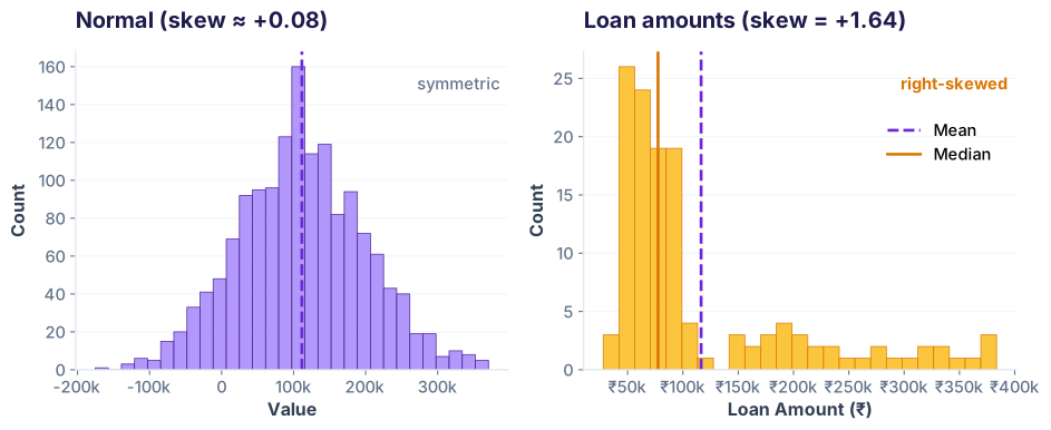
Normal (synthetic) vs the real loan amount distribution (right-skewed)
Two histograms side by side. Left: a symmetric normal distribution (skew near zero). Right: the real loan amount distribution with a long right tail (skew +1.64).
Measure skewness and kurtosis
What this shows: Loan amounts have skewness +1.64 (right tail, pulled up by large loans). Rule of thumb: |skew| > 1 = highly skewed. Kurtosis +1.79 means tails are heavier than a normal curve but not extreme. Diagnostic takeaway: this distribution isn't bell-curve, so report median rather than mean when summarising a typical loan.

Categorical columns: .describe(include='object')

Non-numerical columns (strings, categories) get their own summary: count, unique values, top (most common), and frequency.

Stat employment_type city
count 150 150
unique 3 6
top (most common) Salaried Mumbai
freq 118 33
Describe categorical data
What this shows: 118 of 150 loans are Salaried (79%), with Self-employed (31) and a lone Student (1) rounding out the portfolio. Mumbai leads city-wise with 33 loans, followed by Hyderabad (32), Delhi (29), Bangalore (28), and Pune (27) — a reasonably balanced spread across 6 cities. The freq row flags if one category dominates (risk for bias or seasonal effects); here Salaried concentration is a watchpoint.

Custom percentiles with .quantile()

Percentiles carve data into slices. Use them to spot tail risk: P99 tells you the worst 1% of loans. P1 tells you the best.
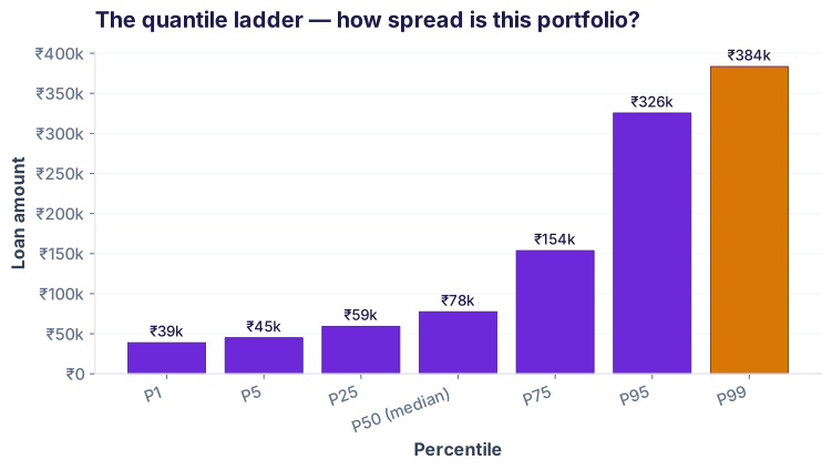
The quantile ladder — how far the top 1% sits above the median
Bar chart of loan amounts at the 1st, 5th, 25th, 50th, 75th, 95th, and 99th percentiles. The P99 bar (highlighted amber) towers over the median.
Percentile Loan Amount Interpretation
P1 (1st percentile) ₹38,870 Bottom 1% of loans
P5 (5th percentile) ₹45,000 Bottom 5%
P50 (median) ₹77,500 Middle 50%
P95 (95th percentile) ₹325,500 Top 5%
P99 (99th percentile) ₹383,550 Top 1% (tail risk)
Calculate custom quantiles
What this shows: The spread is dramatic: P1 (₹38.9k) to P99 (₹383.6k) is a 10× range. Risk officers care about P95 and P99 — if those top 5% loans default, what's the exposure? Here the top 1% alone could be ~₹384k × number of loans in that slice. Median (P50) is ₹77.5k, a safer bet for "typical" loan size.

Next level: Group and describe (Lesson 14 preview)

Descriptive stats become powerful when you segment by employment type, city, or age band. Here's a preview of what groupby unlocks:

Grouped summaries (coming next lesson)
What this unlocks: Salaried employees take the largest loans (mean ₹126k) but have huge spread (std ₹98k). Self-employed are more consistent (mean ₹85k, std ₹35k). The lone Student row shows why tiny groups can't be compared directly. One number can hide stories — groupby reveals them. Next lesson teaches the syntax.
🎯
Check your understanding
Q1: What does a standard deviation of 0 mean?
Every value in the column is identical.
The data is perfectly normally distributed.
The mean equals the median.
There are no outliers in the data.
Q2: When is the median a better summary than the mean?
Always; the median is always better.
When the data is skewed or has outliers.
When the data is perfectly normal.
When you have more than 100 rows.
Q3: What does .describe(include='all') give you that .describe() alone doesn't?
It runs faster.
Summaries of categorical (object) columns like count, unique, top, and freq.
It calculates skewness and kurtosis.
It groups data by employment type automatically.
0
/3
Great start!

You're ready to move to groupby and pivot operations.