You're writing a donor report on immunization outreach coverage in a regional health program. You've surveyed 500 facilities across five districts and recorded mother's age, distance to clinic, household size, and whether children received doses on schedule. Your stakeholders ask: What's the true coverage rate across the whole region? And how confident are you? The mean of your 500 facilities is 68% — but if you repeat the survey, will you get 68% again? Distributions and sampling math give you a 95% confidence interval.
📥
Sample dataset included
500 rows of immunization monitoring data from regional health outreach
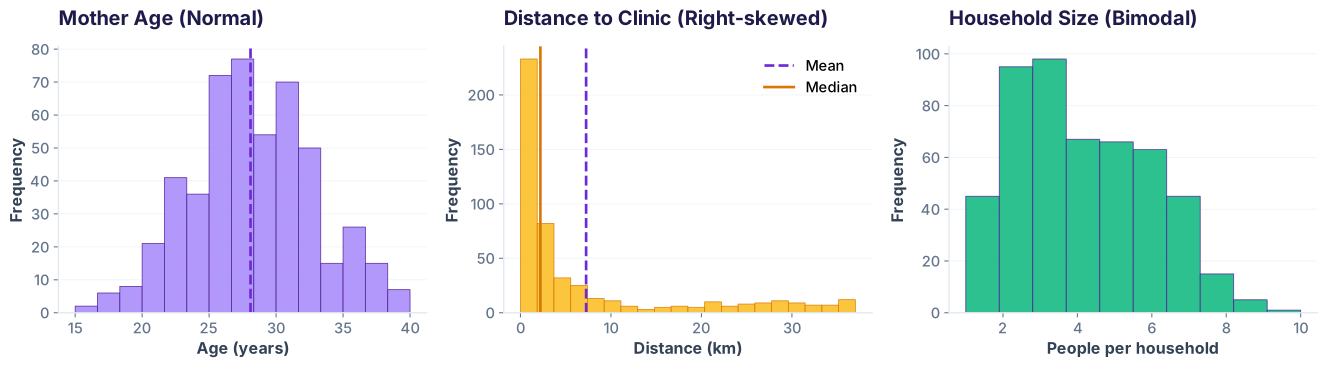
The mean and standard deviation describe a dataset well — but only if the data is shaped like a bell curve. Look at three real columns from your immunization data: they tell three different stories.
Three distributions from the same dataset. Same axes, very different shapes.
What this shows: Mother's age looks like a bell curve — mean 28, std 5 describes it well. Distance has a long tail (right-skew) — most values cluster below 5 km, with outliers to 40 km. Household size shows two peaks (rural ~6 people, urban ~3) — the mean of ~4.5 lies between them, describing neither group. When you see skew or bimodality, you need different tools.
Compute summary stats for each column
The Normal Distribution: 68-95-99.7 Rule
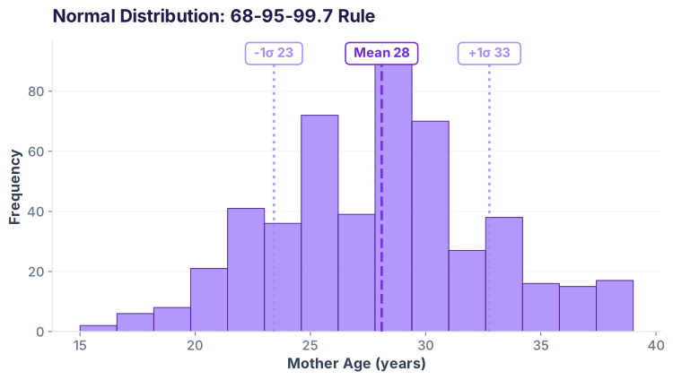
When data follows a bell curve, the standard deviation tells you exactly how much data falls within each band: 68% within 1 std, 95% within 2 std, 99.7% within 3 std. This is your map for interpreting real-world variation.
Mother age histogram with normal curve overlay and the 68-95-99.7 rule visualized.
What this shows: The red dashed line is the mean (28 years). One standard deviation (5 years) on either side covers 68% of your sample. Two standard deviations cover 95%. This rule lets you quickly assess how typical a value is: a 38-year-old mother is still within ±2σ (not unusual), but a 45-year-old is beyond the normal range and worth investigating.
Using scipy.stats.norm to calculate percentiles
Skewed Distributions: When the Tail Wags
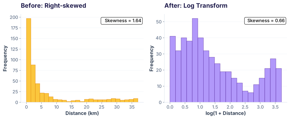
Distance to clinic is right-skewed: most facilities are close (under 5 km), but some outliers sit 40 km away. A log transform can normalize it, making it easier to model and reason about on a linear scale.
Distance to clinic: before and after log transformation. The tail gets pulled in.
What this shows: On the left, the raw distance histogram has a dramatic tail — the tall bar on the left and tiny bars trailing right make it hard to model. After applying np.log1p() (log transform), the distribution is more symmetric. Many statistical models assume normality; the transform allows you to use normal-based methods on skewed data.
Apply log transform to normalize a skewed column
Bimodal & Multimodal Distributions: Segment First
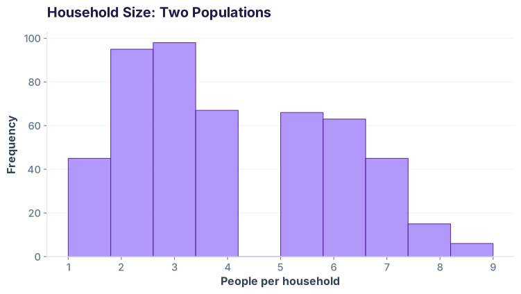
Household size in rural areas averages 6 people; in urban areas, about 3. Your overall mean is 4.5 — but that describes neither group. When you see two peaks, your data is screaming: segment me first!
Household size histogram showing two populations: urban (3-4 people) and rural (5-7 people).
What this shows: Urban facilities cluster around 3–4 household members, rural around 5–7. The histogram shows two distinct peaks. Reporting a single mean (4.5) hides the real pattern. The insight: segment your data by geography first, then compute mean and confidence interval for each group separately. You'll tell a richer story.
Detect and separate bimodal data
The Central Limit Theorem: Magic in One Picture
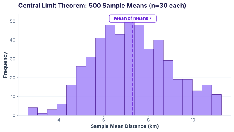
Here's the theorem's power: even if your population is wildly skewed, the means of random samples follow a bell curve. Run a simulation: draw 500 random samples of size 30 from the right-skewed distance column, compute each sample's mean, and plot them.
Simulation: 500 sample means (each from n=30 observations) follow a normal distribution, even though the population is right-skewed.
What this shows: The left histogram is the raw, right-skewed distance data. On the right, we drew 500 random samples of 30 facilities each, calculated the mean of each sample, and plotted those means. They form a bell curve! This is the Central Limit Theorem — one of the most powerful ideas in statistics. It means that even if your raw data is weird, your sample mean will be approximately normal, so you can use normal-based confidence intervals.
Simulate the Central Limit Theorem
Confidence Intervals: Quantifying Your Uncertainty
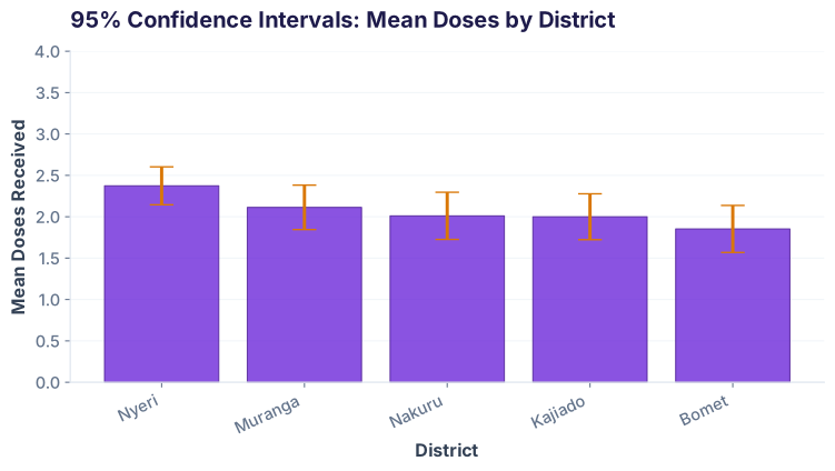
A confidence interval (CI) says: if I repeated this survey 100 times, the true population mean would lie within my calculated range in 95 of those repetitions. For doses_received (which ranges 0–4), we compute a 95% CI.
95% confidence intervals for mean doses across 5 districts. Wider bars = more uncertainty (smaller sample or higher variance).
What this shows: Each dot is the sample mean doses in a district, and the bar around it is the 95% confidence interval. Narrower bars (like Nyeri) mean higher confidence — you have more data or less variability. Wider bars mean more uncertainty. The key insight: if you sampled the same districts 100 times, 95 of those samples' intervals would contain the true population mean.
Compute 95% confidence interval for mean doses
📝
Self-Check Quiz
What does a 95% confidence level actually mean?
If you repeated the survey 100 times, about 95 of the confidence intervals would contain the true population mean.
There is a 95% probability the true mean is inside your interval from this one survey.
95% of your sample data falls within the confidence interval.
The true mean will definitely be in your interval.
Why does the Central Limit Theorem matter for real analysis?
It proves your population is normally distributed.
It allows us to build normal-based confidence intervals even if the population is skewed, because sample means are approximately normal.
It guarantees your sample mean equals the population mean.
It eliminates the need to check data distributions.
When your histogram is bimodal, what should you do?
Report both the mean and the standard deviation — they fully describe the data.
Segment your data by the underlying groups first, then compute summary statistics for each group separately.
Apply a log transform to make it normal.
Ignore the bimodality; it's not important for analysis.
Quiz Complete!
You're ready to build confidence intervals in real donor reports.
Africa & India's Best AI Academy
🤖 AI-first🎓 Placement Assistance
Ready to analyze real-world survey data?
Join the Best AI Program: The AI-Era Analyst — 5 months, fully online, with placement assistance. Week 1 is free.