
Your manager walks over at 9am on Friday: "We need a chart for the CEO deck tomorrow. Six months of daily order volume, with a call-out on Black Friday. Make it look sharp." You have the data (a CSV of 180 days), but you've only ever made basic line charts. You know matplotlib can do better — but the API feels overwhelming. Figure? Axes? Why do I need both? In the next 30 minutes, you'll master the mental model and ship five production-ready charts.
Why Matplotlib? The Fig/Ax Model
Matplotlib is powerful because it separates what you're drawing on (the figure) from what you're drawing (the axes). Most one-liners skip this — they create both behind the scenes. But when you need fine-grained control (custom colors, annotations, multiple plots), you must understand the model.
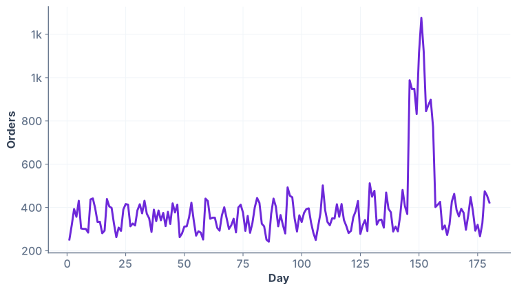
plt.plot(x, y) and plt.show(). It works, but it tells no story and looks unfinished. The CEO would ask: "What is this? What do the axes mean?"
One-liner vs. The Right Way
Compare two approaches:
ax.set_title(), ax.grid(), ax.annotate(). For production work — the kind that lands in a slide deck — always use fig/ax.
Styling Essentials: Title, Labels, Grid, Color
A polished chart has four non-negotiables: a clear title, axis labels, a subtle grid, and brand colors. Let's upgrade the basic line chart with each.
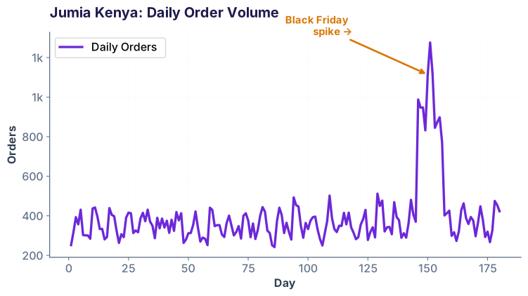
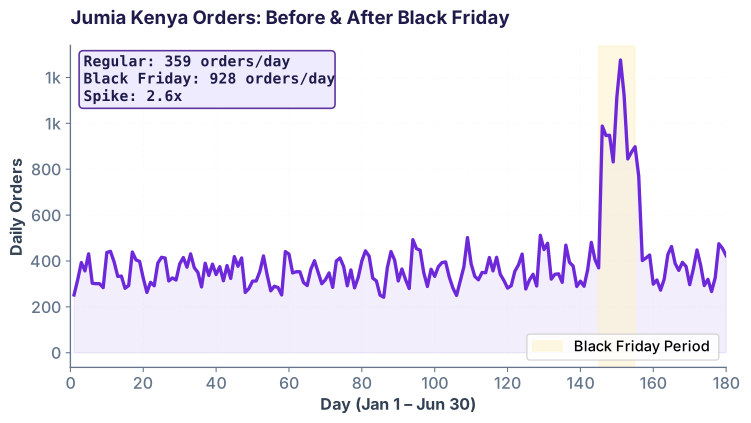
ax.set_title() and ax.set_xlabel() / ax.set_ylabel() to label the axes. Grid lines make it easier to read values. The purple color (#6D28D9) matches Ramayai's brand. The arrow annotation draws attention to the Black Friday spike around day 150 — the moment orders nearly tripled. This is the chart you'd show your manager.
Subplots: Multiple Charts in One Figure
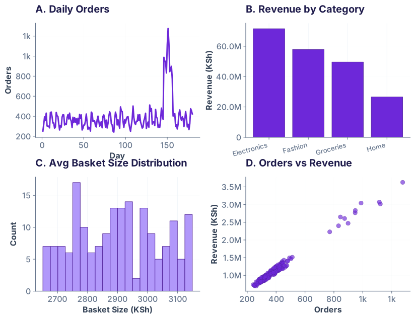
Often you need to show related views side-by-side: orders vs. revenue, distribution of basket sizes, scatter of order volume vs. revenue. Use plt.subplots(rows, cols) to create a grid of axes, then populate each.
Horizontal Bar Charts: When Labels Are Long
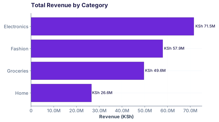
Vertical bar charts are the default, but when your categories have long names or you want to sort by value, horizontal bars are clearer. Use ax.barh() instead of ax.bar().
Annotations & Publication Quality: Before You Ship
The difference between "a chart I made in Jupyter" and "a chart ready for the CEO deck" is attention to detail: highlighted regions, statistics boxes, clean typography, and proper spacing.
Export for Slides & PDF
Once your chart is publication-ready, export it in two formats:
- SVG for web/slides: Vector format, scales without quality loss.
fig.savefig('chart.svg') - PNG (150–300 DPI) for documents: Raster, but high DPI looks crisp in PDFs.
fig.savefig('chart.png', dpi=300) - PDF for print: Vector + text, perfect for reports.
fig.savefig('chart.pdf', dpi=300, bbox_inches='tight')
Common Pitfalls & How to Avoid Them
1. Forgetting tight_layout()
When you have subplots or a complex layout, labels can overlap. Always call fig.tight_layout() before saving or showing.
2. Using bare plt.* instead of ax methods
Mixing plt.plot() (global) with ax.set_title() (on a specific axes) is confusing. Pick one: either all pyplot (plt.*) for simple exploration, or all object-oriented (fig, ax) for production.
3. Not setting figsize early
Size matters. Mobile slide decks want 10×6; printed reports want 8×10. Set figsize when you create the figure: fig, ax = plt.subplots(figsize=(10, 6))
4. Ignoring gridlines or making them too heavy
A grid helps readability, but only if it's subtle. Use ax.grid(True, alpha=0.2, linestyle='--') — light and dashed, never solid or opaque.
5. Skipping axis labels
Never assume your audience knows what the axes mean. Every chart needs ax.set_xlabel() and ax.set_ylabel().
Quick check-in
Ready to make charts people share?
Join the Best AI Program: The AI-Era Analyst — 5 months, fully online, with placement assistance. Week 1 is free.
Explore The AI-Era Analyst →