
You're building a weekly insights deck for the payments leadership team. The default Excel charts look dated. You need to produce publication-ready visuals fast—countplots, distributions, heatmaps—and ship them as SVG or PNG for reports. You also want to explore payment trends interactively before you finalize them.
Why Seaborn? Opinionated defaults that save hours
Matplotlib is the foundation—it's powerful but verbose. Seaborn sits on top and gives you statistical graphics with a single function call. The colours work, the fonts breathe, the proportions feel right.
Seaborn
- Beautiful defaults (no tweaking axis labels)
- Built-in statistical plots (countplot, boxplot, heatmap)
- Easy multi-variable relationships (FacetGrid)
- Integrates seamlessly with pandas
- SVG/PNG export for reports
Plotly
- Interactive (hover, zoom, click legends)
- Dashboards in Streamlit or Dash
- 3D charts and animations
- Great for exploration & demos
- HTML export (can't use in PDF reports)
The pattern: Use Seaborn for static reports, Plotly for interactive dashboards. Sometimes you'll use both in the same workflow.
Countplot: Category frequencies at a glance
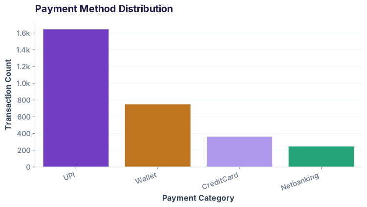
Payment methods aren't equally distributed. UPI dominates. A countplot shows the picture in one chart:
Boxplot: Distributions across groups
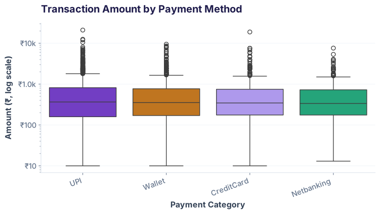
Amounts vary wildly by payment method. A boxplot shows median, quartiles, and outliers side-by-side:
Heatmap: Two-way relationships
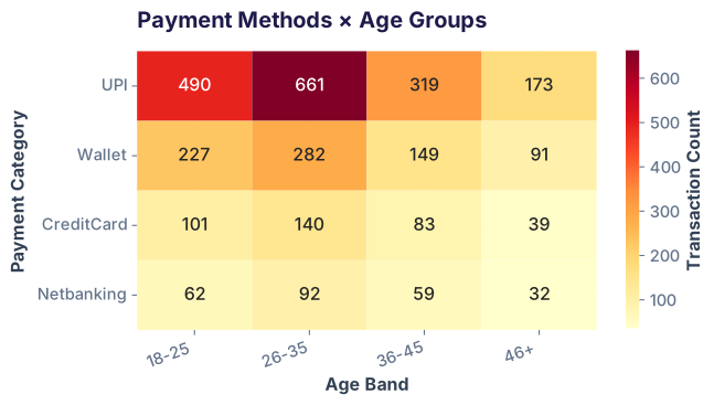
How do payment methods vary by age group? A heatmap shows the intersection counts as color intensity:
FacetGrid: Small multiples for clarity
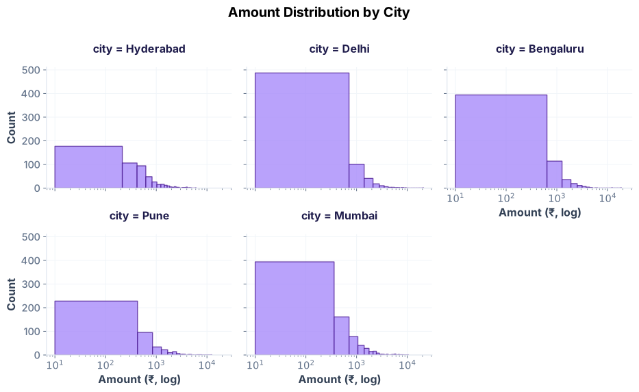
Same chart, separate panels for each city. FacetGrid repeats a plot across subgroups:
When to use Plotly: Interactive exploration
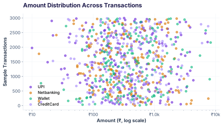
Plotly shines when you need interactivity. Hover to see exact values, click legends to toggle series, zoom into clusters. Perfect for dashboards and live demos.
Exporting to SVG & PNG for reports
Both libraries ship static formats. For Seaborn (matplotlib), use savefig() with format. For Plotly, use kaleido (requires headless browser):
Common pitfalls & how to avoid them
1. Forgetting to scale log axes for right-skewed data
Transaction amounts are lognormal. A linear y-axis squashes most data near zero. Always use plt.yscale('log') or fig.update_yaxes(type='log').
2. Too many colours in a heatmap
Sequential palettes (single-hue gradients) work best. Avoid rainbow or diverging colormaps unless you're showing negative correlations.
3. Forgetting to use tight_layout()
Labels often get cut off at export. Always call plt.tight_layout() before savefig().
4. Overloading FacetGrid with too many subplots
A 5×5 grid of histograms becomes unreadable. Stick to 6–12 subplots max. If you have more categories, use colour or interactivity (Plotly) instead.
5. Trying to use Plotly HTML in a PDF report
Plotly HTML files don't embed in PDFs. Export to PNG or SVG if the output must be static.
Quick reference: Seaborn vs. Plotly
| Use Case | Seaborn | Plotly |
|---|---|---|
| Statistical plots (countplot, boxplot, heatmap) | ✓ Native functions | ⚠ Requires custom code |
| Static reports (PDF, Word) | ✓ SVG/PNG export | ⚠ Needs kaleido |
| Interactive dashboards | ✗ Static only | ✓ Native HTML |
| Exploration in Jupyter | ✓ Fast iteration | ✓ Great hover info |
| Small file size | ✓ SVG compact | ⚠ HTML can be large |
| Learning curve | ✓ Gentle (if you know matplotlib) | ⚠ Steeper (different API) |
Ready to let stakeholders click?
Join the Best AI Program: The AI-Era Analyst — 5 months, fully online, with placement assistance. Week 1 is free.
Explore The AI-Era Analyst →