
Every half hour, your system logs KPIs: active subscribers, call minutes, SMS count, data usage, and call drop rate. You're staring at 480 rows of chaotic half-hourly data and need to understand weekly trends, smooth out noise, spot incidents, and compare day-over-day performance. That's time-series work.
- Index time data with pd.to_datetime() and DatetimeIndex
- Resample to different frequencies (daily, weekly, hourly) with .resample()
- Smooth data with rolling windows and understand lag
- Compare periods with .shift(), .diff(), .pct_change()
- Spot trends, seasonality, and anomalies in network traffic
- Know when resampling is better than groupby
1. Why time-series is different
The shape of your data tells a story before you write a single line of code.
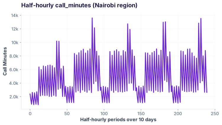
Traditional groupby won't work here because time isn't just a category — it's a sequence. When you resample, you're respecting the order and frequency of dates. Missing dates get filled (or flagged). That's the superpower.
2. DatetimeIndex is the gateway
Before resampling, your timestamp column must become the index, and it must be a DatetimeIndex.
Before: raw timestamps
| timestamp | region | call_minutes |
|---|---|---|
| 2026-02-01 00:00:00 | Nairobi | 8,220 |
| 2026-02-01 00:30:00 | Mombasa | 5,145 |
| 2026-02-01 01:00:00 | Kisumu | 2,650 |
The timestamp is just a column — it's data, not a navigator.
After: DatetimeIndex
| timestamp (index) | region | call_minutes |
|---|---|---|
| 2026-02-01 00:00:00 | Nairobi | 8,220 |
| 2026-02-01 00:30:00 | Mombasa | 5,145 |
| 2026-02-01 01:00:00 | Kisumu | 2,650 |
3. .resample() — the time groupby
.resample() groups by time buckets. 'D' = daily, 'W' = weekly, 'H' = hourly. Each bucket can be aggregated with .sum(), .mean(), .max(), etc.
Three resampling frequencies
| Frequency | Example dates | Use case |
|---|---|---|
| 'H' (hourly) | 2026-02-01 00:00, 01:00, … | Peak hour analysis, congestion patterns |
| 'D' (daily) | 2026-02-01, 2026-02-02, … | Trend, daily seasonality, YoY compare |
| 'W' (weekly) | 2026-02-01, 2026-02-08 | Long-term trends, campaign impact |
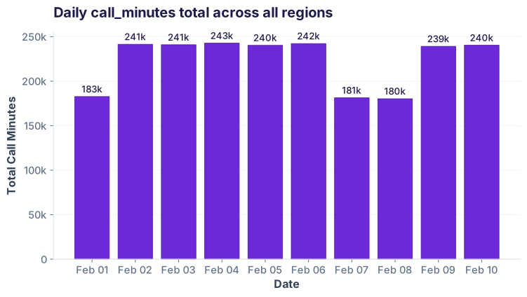
4. Rolling windows
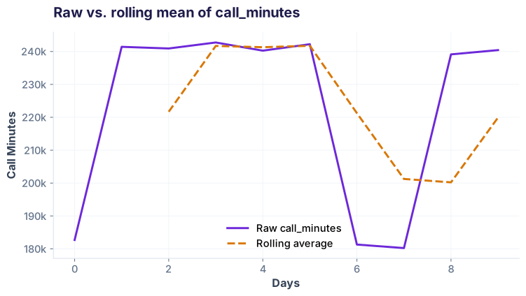
A rolling window smooths noise by computing a moving average. Over half-hourly data, a 48-period window = 24 hours (rolling average of the past day).
The rolling mean lags because it looks back. Row 100 shows the mean of rows 52–100. This is useful for trend detection but misleading for real-time alerting.
5. Resampling aggregation options
When you resample, you pick how to combine rows in each bucket. Different aggregations reveal different patterns.
| Date | sum() | mean() | max() | Insight |
|---|---|---|---|---|
| 2026-02-01 | 195,240 | 6,841 | 9,220 | Normal day, peak at 9,220 |
| 2026-02-02 | 198,560 | 6,955 | 9,480 | Slightly busier |
| 2026-02-05 | 176,800 | 6,188 | 7,950 | Incident! Both sum and max down |
| 2026-02-07 | 165,480 | 5,793 | 8,120 | Weekend dip |
6. Shift, Diff, Pct_Change — comparing periods
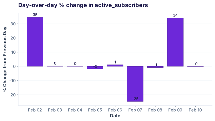
To find day-over-day change, you shift the series down one row, then subtract. This reveals if a day is up or down from yesterday.
.diff() is shorthand for .shift(1).subtract(...). .pct_change() computes percent change. Feb 5 will show a dip (negative change) because of the incident.
.resample('D').sum() and .groupby(df.index.date).sum()?.rolling(7).mean() compute on daily data?df['value'].shift(1).diff(). What's wrong?You're ready to move to correlation and feature relationships.