
NeoBank's risk team in Mumbai uses machine learning to decide which loan applicants will default. But here's the problem: when a regulator asks "Why did you deny this person's ₹50,000 loan?", a logistic regression coefficient doesn't cut it. They need to hear: "This person's credit score is 520, which is below our threshold of 580. Applicants in that range default 65% of the time."
That's where decision trees shine. They make plain-language rules. A tree reads like a flowchart: "If credit_score ≤ 580 AND loan_amount > ₹80,000, then high default risk." Every decision is explainable, auditable, and defensible to regulators.
Why decision trees? Three reasons
Logistic regression and neural networks are black boxes. Decision trees are transparent.
2. No scaling needed. Trees split on thresholds, not distances. ₹10,000 and ₹1 million are equally readable. StandardScaler? Not required.
3. Handles mixed data. Numeric, categorical, missing values — trees handle all of it. No LabelEncoder, no one-hot encoding fuss.
The cost: trees tend to overfit. A deep tree memorizes the training data instead of learning patterns. We'll tackle that with pruning.
How splitting works: the tree algorithm
A decision tree grows by asking a series of yes/no questions. At each node, it picks a feature and a threshold, splitting the data to maximize purity (homogeneity of class labels).
Start at the root. All 10,000 applicants. Mix of defaulters (40.5%) and non-defaulters (59.5%). The algorithm asks: "Which single feature and threshold best separates defaulters from non-defaulters?" Answer: credit_score ≤ 580 splits the data the cleanest. Left branch gets high-risk applicants, right gets low-risk.
Then repeat. In the left branch (credit_score ≤ 580), ask again: what's the next best split? Maybe employment_years ≤ 2? Each split reduces impurity (the mixture of classes) until nodes become pure or we hit depth limits.
Gini impurity: measuring node purity
How does the tree know which split is "best"? It measures impurity with a metric called Gini impurity.
Gini ranges from 0 (pure: all one class) to 0.5 for binary (impure: 50/50 split). The tree tries to find splits that reduce Gini the most.
Entropy: an alternative to Gini
Entropy is another purity metric. Scikit-learn supports both.
Both Gini and Entropy work well. Gini is faster (no logarithms). In practice, they give nearly identical results. We'll use Gini (the default) unless specified otherwise.
Training a decision tree with scikit-learn
Let's build a tree on NeoBank's credit data. Start simple: no depth limit. Watch it overfit.
Perfect training accuracy (1.0) but test accuracy drops to 0.62. The tree has 45 levels and 2,468 leaf nodes — it's memorizing. We need to prune.
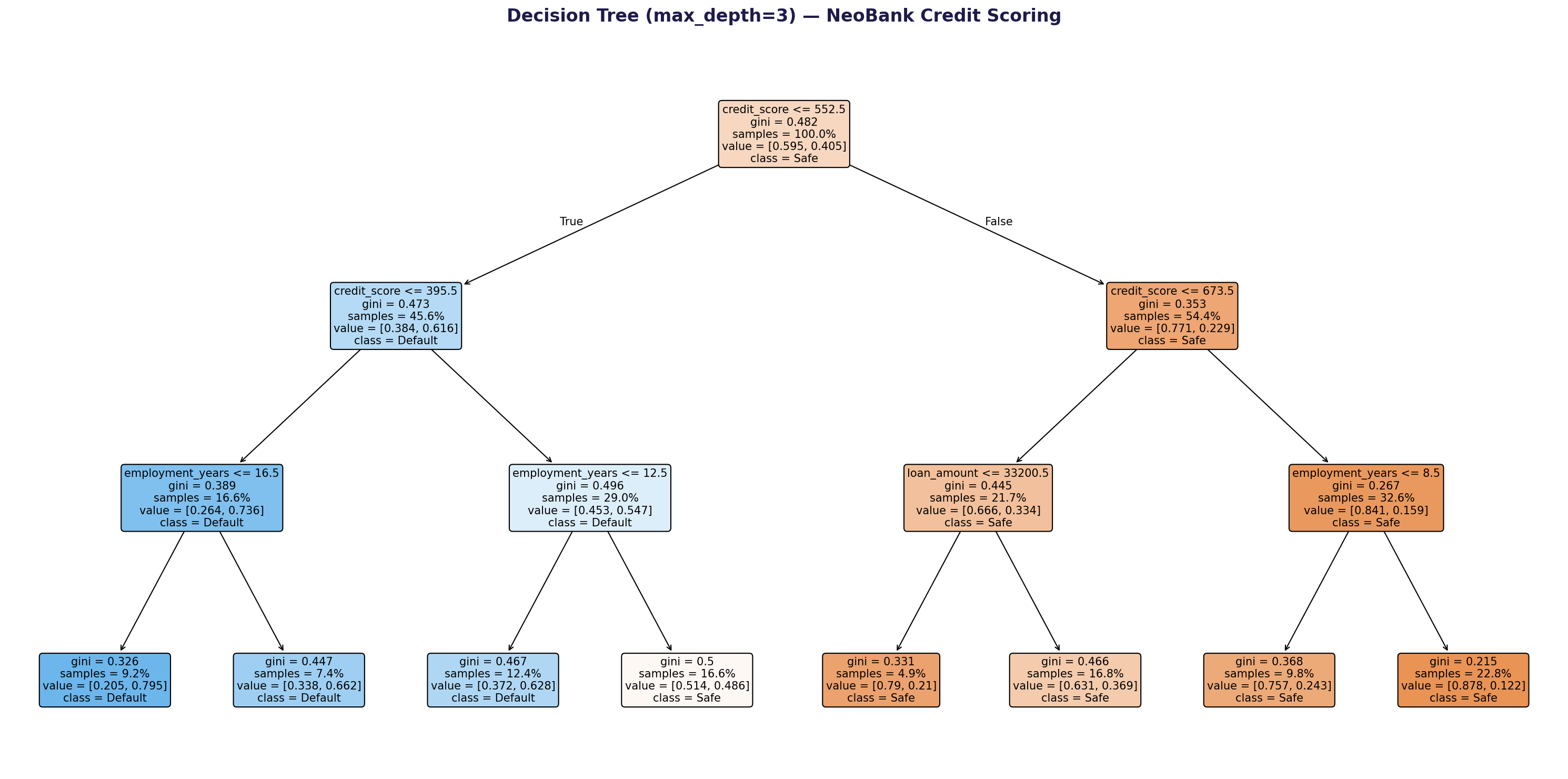
Visualizing the tree (pruned to depth 3)
Feature importance: which features matter most?
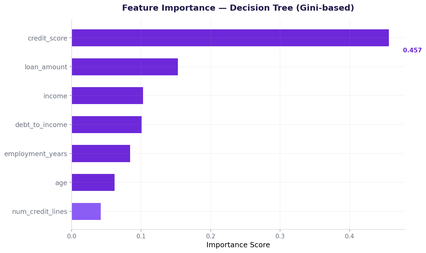
After training, the tree tells us which features it relied on. Credit score dominates.
Credit score captures 79% of the tree's decision-making. That makes sense: it's the strongest predictor of default. Loan amount and employment years contribute next.
Overfitting with depth: the critical experiment
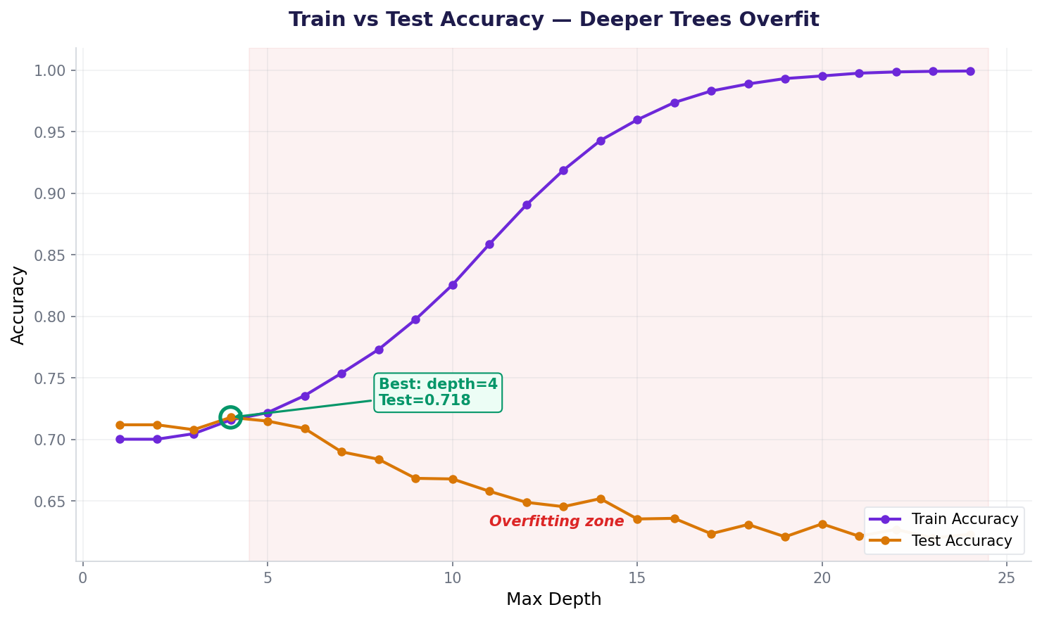
Shallow trees underfit (miss patterns). Deep trees overfit (memorize noise). Let's find the sweet spot.
Notice the pattern:
- Depth 3: Underfitting. Train and test are close but both are low (0.704 and 0.708).
- Depth 5: Just right. Test peaks at 0.712. Train and test gap is small (0.01).
- Depth 7+: Overfitting. Train rises (0.754, 0.833) but test drops (0.690, 0.662). The gap widens.
- Depth None: Severe overfitting. Train = 1.0 (memorized), test = 0.618 (worse than depth 3).
Pruning: the levers to prevent overfitting
Decision trees have three main pruning levers in scikit-learn. Use them together.
max_depthmax_depth=5min_samples_splitmin_samples_split=20min_samples_leafmin_samples_leaf=10With pruning: depth 5, 32 leaves. Clean, interpretable, and performant on test data (0.712 accuracy). This is the tree we'd show to a regulator.
Understanding tree structure: from root to leaf
A decision tree's power is that you can trace any prediction. For an applicant with credit_score=520 and loan_amount=₹90,000, the tree would navigate:
Left child: "Is employment_years ≤ 2?" → Yes, go left (very high-risk)
Left leaf: "Predict: Default" (65% defaulters in this leaf)
Result: This applicant is flagged as likely to default because they have low credit score (520) AND short employment (1 year). You can show this path to the regulator.
Scikit-learn has a function to visualize trees:
For a depth=3 tree, the visualization is compact. At each node, you see: the split condition (feature and threshold), the Gini impurity, the sample count, and the class distribution.
Also used in...
Domain Spotlight
How AI systems use this
Decision trees are the building blocks of modern machine learning. Random Forest (Lesson 12) is 100 trees voting together. XGBoost (Lesson 13) trains trees sequentially, each correcting the previous one's errors. Gradient Boosting, LightGBM, and CatBoost all build on this foundation. Every tree-based model you'll encounter relies on the splitting, Gini, and pruning concepts from this lesson.
Task: Load credit_default.csv. Train decision trees with depths 1, 3, 5, 7, 10. For each, compute test accuracy and the train-test gap. Which depth minimizes overfitting while maximizing test accuracy? Print the results in a table.
Hint 1: Use a loop: for depth in [1, 3, 5, 7, 10]:
Hint 2: For each depth, create a DecisionTreeClassifier and fit on train data
Hint 3: Use accuracy_score(y_test, dt.predict(X_test)) to get test accuracy
Hint 4: Gap = train_accuracy - test_accuracy. A small gap (< 0.05) is good; a large gap (> 0.15) signals overfitting.
Interview questions: test your understanding
Quiz: 5 questions to test your knowledge
Cheatsheet: decision trees at a glance
| Concept | What it does | Code |
|---|---|---|
| Gini impurity | Measures node purity | criterion='gini' |
| Entropy | Alternative purity measure | criterion='entropy' |
| max_depth | Limits tree height | max_depth=5 |
| min_samples_split | Min samples to allow split | min_samples_split=20 |
| min_samples_leaf | Min samples per leaf | min_samples_leaf=10 |
| feature_importances_ | Which features matter most | dt.feature_importances_ |
| get_depth() | Check final tree height | dt.get_depth() |
Common mistakes: what breaks and how to fix it
class_weight='balanced' to penalize minority class errors more heavily.Key takeaways
Decision trees are your window into machine learning. Everything that follows—Random Forests, XGBoost, Gradient Boosting—is built on these foundations.
- Interpretability matters. A tree's rule "If credit_score ≤ 580 AND loan_amount > ₹80,000, then default" is worth its weight in regulatory compliance.
- Gini impurity guides splits. Lower Gini = purer node. The tree recursively finds splits that minimize Gini the most.
- Depth controls overfitting. Deep trees memorize. Shallow trees miss patterns. Find the sweet spot with train-test comparison.
- Prune aggressively. Use max_depth, min_samples_split, and min_samples_leaf together. A smaller tree is almost always better than a deep one.
- Feature importance is a hint, not gospel. One tree is biased. Use ensembles to confirm which features truly matter.
Ready to build explainable AI?
Join the Best AI Program: The AI-Era Analyst — 5 months, fully online, with placement assistance. Week 1 is free.
Explore The AI-Era Analyst →