
Amara is a data scientist at TelcoMax, a telecom in Nairobi. She has a preprocessed dataset of 5,000 customers with 19 features (after one-hot encoding: service type, contract length, internet options, device categories). She wants to:
- Visualize customer groups in 2D to understand churn patterns. But 19D plots are impossible.
- Speed up model training. Fewer features = faster fitting and less overfitting risk.
- Reduce noise. Some features are correlated; PCA isolates signal.
PCA solves this: compress 19 features into uncorrelated principal components. Keep the top 2 for plotting (captures 18.25% of variance), or the top 15 for modeling (captures 90%).
What is PCA? Finding directions of maximum variance
Principal Component Analysis (PCA) answers: "In which directions does my data vary the most?" Instead of keeping all original features, PCA creates new features (principal components) that are uncorrelated and ordered by how much variance they explain.
Result: You can keep the first k components (e.g., 2 or 15) and drop the rest without losing much information.
Why is this useful? Fewer features mean faster training, less overfitting, easier visualization, and cleaner signal (by discarding noise-heavy components).
Eigenvalues and eigenvectors: the math intuition
PCA relies on two concepts from linear algebra:
- Eigenvector: A direction (vector) in your feature space. For PCA, each eigenvector of the covariance matrix is a principal component direction.
- Eigenvalue: A number telling you how much variance is explained along that eigenvector direction. Larger eigenvalue = more variance = more important principal component.
When you compute PCA on your data, scikit-learn's PCA().fit(X) finds the covariance matrix, computes its eigenvalues (and eigenvectors), and sorts them by magnitude (largest first). The eigenvalues directly tell you the explained variance per component.
Explained variance ratio: which components to keep?
Each component explains a percentage of total variance. The "explained variance ratio" is individual component variance divided by total. The "cumulative explained variance" sums these up.
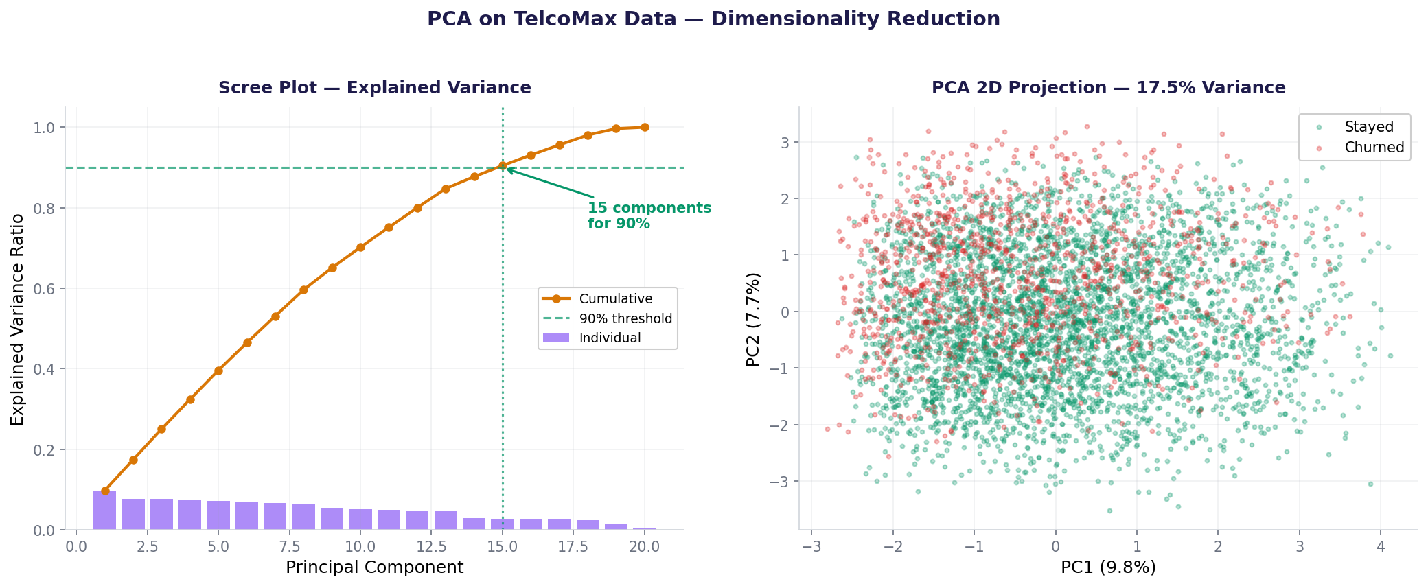
Key insights: PC1 alone captures 10.23%. The first 2 components together capture 18.25%—enough to visualize 5,000 customers in 2D. For modeling, we need 15 components to retain 90% of variance.
Scree plot: visualizing variance drop-off
A scree plot shows the explained variance ratio for each component. You're looking for the "elbow"—where variance drops sharply. Keep components before the elbow.
Cumulative variance: deciding how many components
The cumulative variance plot shows total variance retained by the first k components. Use this to decide: Do I want 90%? 95%? The steeper the initial climb, the better—fewer components needed.
PCA for visualization: compress to 2D
Humans can't see in 19 dimensions. PCA(n_components=2) gives you a 2D view of your data.
You've compressed 19 features to 2, retaining 18.25% of variance. The plot lets you spot clusters, outliers, or class separation. For churn prediction, you might see churned customers clustering away from retained ones.
PCA for modeling: reduce features, keep 90%
For training a classifier, you typically want more variance retained (90%+) than for visualization.
The model achieves 80.57% accuracy on test data with fewer features. PCA speeds up training and often improves generalization by removing noise-heavy low-variance components.
PCA limitations: it's linear, interpretability is hard
PCA is powerful but has important limits:
- Linear only: PCA finds linear combinations of original features. If your data has nonlinear structure (e.g., a spiral, nested clusters), PCA won't capture it well. Use t-SNE, UMAP, or autoencoders for nonlinear data.
- Interpretation: Each PC is a mix of all original features. You can't easily say "PC1 = customer age + tenure." You need to check the component loadings (eigenvector values).
- Assumes normalization: Outliers or large-scale variables dominate PCA. Always standardize your data before PCA.
- Variance ≠ Usefulness: High-variance features might not be predictive for your target. PCA ignores the target, so an uninformative but high-variance feature gets a high PC ranking.
For supervised learning (classification, regression), consider supervised alternatives like Linear Discriminant Analysis (LDA) or PLS regression.
Understanding component loadings: which features matter?
To interpret what each PC represents, examine the loadings (coefficients). For example, pca.components_[0] shows how much each original feature contributes to PC1.
Notice: Customers with one-year contracts, DSL internet, and security add-ons push PC1 high. Those with month-to-month, fiber, and fewer add-ons push it low. PC1 roughly separates long-term, committed customers from short-term, minimal-service ones.
Also used in...
Domain Spotlight
How AI systems use this
PCA is foundational to machine learning pipelines. Before training deep neural networks, researchers often apply PCA to compress input features, speeding up backpropagation. Autoencoders are a nonlinear extension of PCA, learning hierarchical feature compression. Even large language models use dimensionality reduction internally—transformers project embeddings to lower dimensions for efficiency and to reduce overfitting on noisy words.
Task: Load the sklearn wine dataset (178 samples, 13 features). Fit PCA. Print the explained variance ratio for the first 3 components. Then fit PCA(n_components=2), transform the data, and plot the 2D scatter (color by wine class). How much variance do the first 2 PCs capture?
Hint 1: from sklearn.datasets import load_wine; wine = load_wine(); X = wine.data
Hint 2: pca = PCA(); pca.fit(X); print(pca.explained_variance_ratio_[:3])
Hint 3: pca2 = PCA(n_components=2); X_pca = pca2.fit_transform(X)
Hint 4: Plot: plt.scatter(X_pca[:, 0], X_pca[:, 1], c=wine.target)
Interview questions: test your understanding
Quiz: 5 questions to test your knowledge
Cheatsheet: PCA at a glance
| Task | Code | Output/Use |
|---|---|---|
| Fit PCA | pca = PCA(); pca.fit(X) |
Learns covariance structure |
| Transform data | X_pca = pca.transform(X) |
Projects X to PC space |
| Fit & transform | X_pca = pca.fit_transform(X) |
Combined in one step |
| Get variance (ratio) | pca.explained_variance_ratio_ |
[0.1023, 0.0802, ...] per component |
| Cumulative variance | np.cumsum(pca.explained_variance_ratio_) |
[0.1023, 0.1825, ...] running total |
| 2D visualization | PCA(n_components=2).fit_transform(X) |
(N, 2) array for scatter plot |
| Specify variance % | PCA(n_components=0.90) |
Auto-selects k to reach 90% |
| Get loadings | pca.components_[0] |
Feature contributions to PC1 |
Common mistakes: what breaks and how to fix it
Key takeaways
PCA is a foundational technique for compressing data, visualizing high-dimensional patterns, and speeding up models.
- PCA finds uncorrelated directions (PCs) ranked by variance. The first PC captures the most variance, the second captures the most residual, and so on.
- Explained variance ratio tells you what % each PC explains. Use cumulative variance to decide: 2 components for visualization (18%), 15 for modeling (90%).
- Scree plots and cumulative variance plots help you choose k. Look for the elbow or a threshold (90%, 95%).
- Always standardize before PCA. Scale-dependent variables skew the analysis.
- PCA is linear—good for correlated features, not nonlinear patterns. For nonlinear data, try t-SNE, UMAP, or autoencoders.
- Split data before fitting PCA to avoid leakage. Fit on train, transform test with the same PCA.
- High variance ≠ predictive. For supervised tasks, use LDA or inspect component–target correlation.
Ready to reduce dimensions and accelerate ML?
Join the Best AI Program: The AI-Era Analyst — 5 months, fully online, with placement assistance. Week 1 is free.
Explore The AI-Era Analyst →