
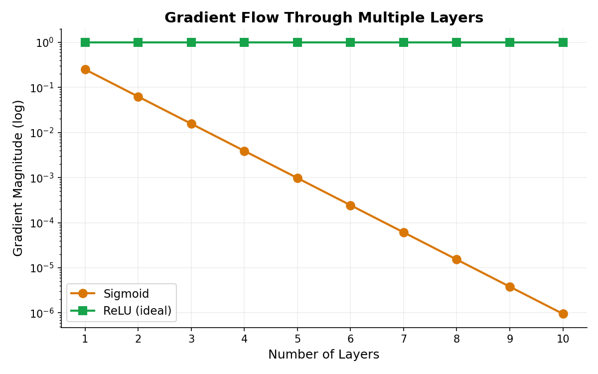
Rebecca is a deep learning engineer at NovaPay, a Bangalore fintech building fraud detection systems. She's designing a network that processes transactions through 10 hidden layers—deep enough to capture complex fraud patterns but not so deep that training becomes impossible. She decides to run an experiment: train two identical networks with different activation functions. First network: sigmoid activation in all hidden layers. Second network: ReLU activation. The results shock her. The sigmoid network barely learns beyond the first few layers. The ReLU network trains smoothly, gradients flowing backward at full strength. She digs deeper into the math: sigmoid gradients decay exponentially (0.25 raised to the power of 10 layers = 0.0000009537), while ReLU maintains constant gradient of 1.0 through all layers. This single architectural choice—the activation function—determines whether her fraud model can be deep or shallow.
What is an activation function?
An activation function is a non-linear transformation applied after each layer's weighted sum. Without it, stacking linear layers is useless—you'd just get another linear transformation. Activations introduce non-linearity, letting neural networks learn complex patterns: curves, jumps, interactions between features. The activation you choose affects three things: (1) how quickly gradients flow backward during training, (2) computational cost, and (3) the range of outputs your neurons produce.
Sigmoid: the classic S-curve
The sigmoid function σ(z) = 1 / (1 + e^-z) squashes any input to a value between 0 and 1. Intuitive for probabilities, widely used in early neural networks.
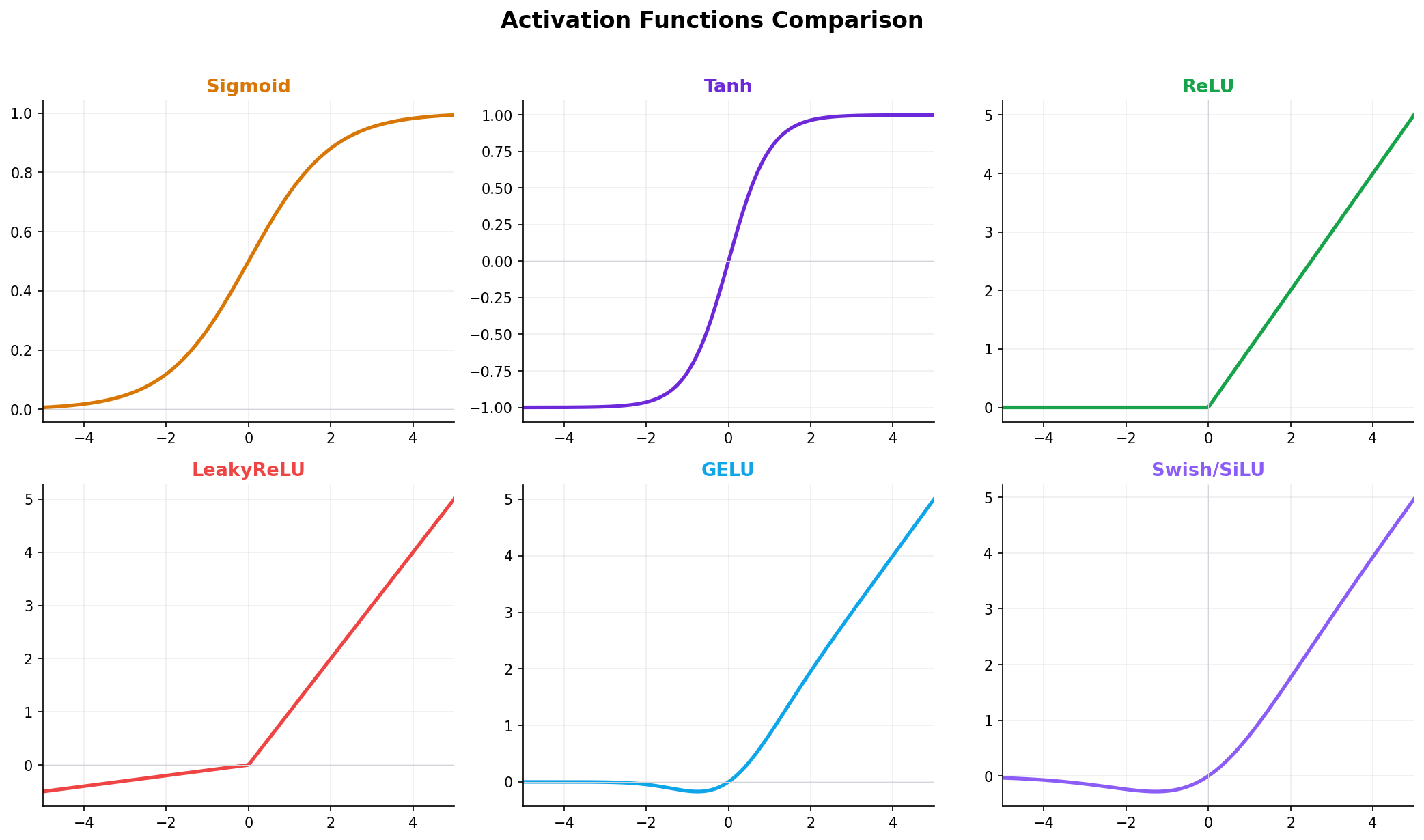
Sigmoid gradient fact: The maximum gradient of sigmoid is 0.25 (at z=0). Once z moves to ±5, the gradient drops to ~0.00665. This is called saturation—the curve flattens, gradients vanish. For deep networks, this is catastrophic.
Tanh: zero-centered sigmoid
Tanh (hyperbolic tangent) is sigmoid's cousin, squashing to -1 to 1 instead of 0 to 1. Slightly better gradient properties (max = 1.0 instead of 0.25), but still suffers from saturation at extreme values.
Why tanh was better: Max gradient of 1.0 (vs sigmoid's 0.25) meant slightly faster training. Zero-centered output (-1 to 1) helped optimization. But still saturates. Rarely used now.
ReLU: the revolution (2011)
Rectified Linear Unit: f(z) = max(0, z). Dead simple. If z is positive, output z. If z is negative, output 0. This single change unlocked deep learning.
Why ReLU changed everything: The gradient is either 1 (if z > 0) or 0 (if z < 0). No saturation curve. This meant that in backpropagation, gradients don't shrink layer by layer. A 50-layer network could train the same way as a 2-layer network. ReLU is also cheap to compute: just a comparison and max operation. It enabled AlexNet (2012, 8 layers) when sigmoid networks maxed out at 2–3 layers.
Leaky ReLU: fixing the dying problem
ReLU has one downside: if a neuron's weights push most inputs to be negative, it outputs 0 forever, with zero gradient. The neuron "dies." Leaky ReLU allows a small negative gradient (typically 0.1 × z when z < 0) to keep gradients flowing.
In practice: Leaky ReLU rarely makes a measurable difference, but it's theoretically safer. Use it if you see dead neurons in ReLU. Most practitioners just use ReLU and move on.
GELU: the transformer activation
Gaussian Error Linear Unit: GELU(z) = z × Φ(z) where Φ is the cumulative distribution function of the standard normal distribution. Smooth, non-monotonic, used in BERT, GPT-2/3, and modern transformers.
Why transformers use GELU: The smooth curve (no sharp corners like ReLU) helps optimization. GELU is slightly more computationally expensive, so it's reserved for large models where the benefit justifies the cost.
Swish / SiLU: self-gated activation
Swish (also called SiLU): f(z) = z × sigmoid(z). Self-gated (sigmoid acts as a gate), smooth, used in EfficientNet and GPT-3.
Self-gating idea: The sigmoid acts as a soft gate. When z is large and positive, sigmoid ≈ 1, so Swish ≈ z. When z is large and negative, sigmoid ≈ 0, so Swish ≈ 0. Smooth transition, good gradient flow.
Gradient strength: why ReLU dominates
Now for Rebecca's critical finding. In backpropagation, gradients are multiplied layer by layer. With sigmoid, each layer multiplies by ≤ 0.25. With ReLU, each layer multiplies by 1.0. Over 10 layers, the difference is catastrophic.
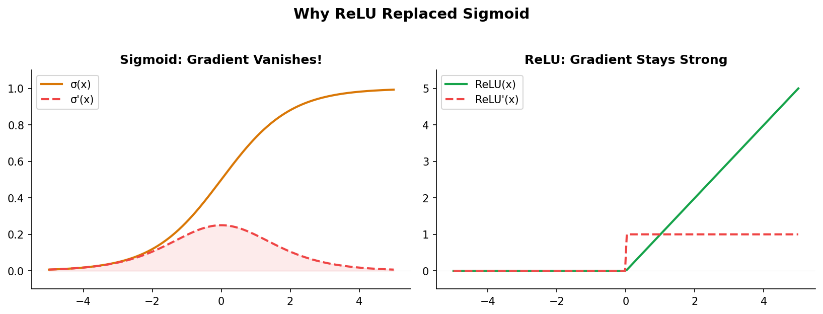
The vanishing gradient phenomenon
This is the core problem Rebecca discovered. Sigmoid gradients don't just get small—they decay exponentially. Let's trace it layer by layer.
The ReLU revolution: before vs after 2012
Before ReLU (pre-2012): Best networks had 2-3 hidden layers. Sigmoid gradients vanish. Researchers stuck with shallow architectures. Feature engineering dominated (manually designing inputs). Training 5+ layer networks was practically impossible.
After ReLU (2012+): AlexNet uses 8 layers and wins ImageNet spectacularly. Suddenly, deep architectures train. Within years: 50-layer ResNets, 100-layer DenseNets, 1000+ layer Transformers (with careful training tricks like residual connections and layer norm). The field shifted from shallow + manual features to deep + learned representations.
The lesson: A small architectural choice (activation function) changed the trajectory of deep learning. ReLU was so effective that it's still the default 13 years later.
Modern activation choice guide
| Use Case | Recommended | Why |
|---|---|---|
| Hidden layers (default) | ReLU | Fast, simple, reliable. Proven to work for CNNs, MLPs, old architectures. |
| Transformers (BERT, GPT) | GELU | Smooth gradient flow. Slightly better for large models. Standard in language models. |
| EfficientNet, modern CNNs | Swish / SiLU | Self-gating helps with feature modulation. Used by Google, works well at scale. |
| Binary classification output | Sigmoid | Squashes to [0, 1], interpretable as probability. Only for output layer. |
| Multi-class output | Softmax | Produces probability distribution across classes. Only for output layer. |
| Regression output | Linear (no activation) | No activation needed. Output is unbounded. |
Practical rule: Start with ReLU for hidden layers. Try GELU if you're building a large transformer. Don't overthink it—activation choice rarely dominates performance compared to other factors like architecture, learning rate, and training data.
How AI systems use this
Activation functions are the invisible foundation of every neural network. Sigmoid was the de facto choice until 2012—researchers couldn't build deep networks, so they engineered shallow ones with hand-crafted features. ReLU unlocked depth. The explosion of deep learning (2012–present) is directly enabled by this single activation. Every CNN, RNN, Transformer, and LLM depends on ReLU or its successors (GELU, Swish). Rebecca's fraud detector at NovaPay will use ReLU in hidden layers and sigmoid or softmax at the output to produce a fraud probability. The choice of activation is so fundamental that getting it wrong (e.g., sigmoid in hidden layers) can make training impossible without obviously breaking anything in the code.
Also used in...
Domain Spotlight
Task: Build a 5-layer neural network on MNIST (digit classification) with three hidden layers. Train it twice: once with ReLU, once with Sigmoid in hidden layers. Measure training loss over 10 epochs. Which converges faster? Why?
Hint 1: Use PyTorch: nn.Sequential(nn.Linear(784, 128), nn.ReLU(), ...)
Hint 2: For sigmoid version, replace nn.ReLU() with nn.Sigmoid()
Hint 3: Plot training loss. ReLU will show steady decrease. Sigmoid will plateau early.
Expected: ReLU converges in 3-4 epochs. Sigmoid barely improves after epoch 2 due to vanishing gradients.
Interview questions: test your understanding
Quiz: 5 questions to test your knowledge
Cheatsheet: activation functions at a glance
| Activation | Formula | Gradient | Best For | Downside |
|---|---|---|---|---|
| Sigmoid | 1 / (1 + e^-z) |
≤ 0.25 | Output layer (binary) | Vanishes in deep networks |
| Tanh | (e^z - e^-z) / (e^z + e^-z) |
≤ 1.0 | Hidden layers (rare now) | Still saturates, slower than ReLU |
| ReLU | max(0, z) |
1 or 0 | Hidden layers (standard) | Dying ReLU (rare) |
| Leaky ReLU | max(αz, z), α≈0.1 |
α or 1 | Hidden layers (safe) | Minimal difference from ReLU |
| GELU | z × Φ(z) |
~1 (smooth) | Transformers (BERT, GPT) | Slightly slower computation |
| Swish / SiLU | z × sigmoid(z) |
Smooth | Large models (EfficientNet, GPT-3) | More complex than ReLU |
Common mistakes: what breaks and how to fix it
You've seen why ReLU changed deep learning.
Now apply it to real production models.
Join the Best AI Program: The AI-Era Agentic Engineer — 5 months, fully online, with placement assistance. Week 1 is free.
Explore The AI-Era Agentic Engineer →