
Kwame is an NLP researcher at Accra Digital Labs, tasked with building a real-time translation system for Twi (Akan language spoken in Ghana) to English. The system needs to understand which source words are relevant for each target word—a task where LSTMs struggle because they compress entire sequences into single vectors.
Kwame discovers the solution: attention. Instead of relying on one vector, the model learns to focus on different parts of the input for each output token. But basic attention (additive) is slow. He needs scaled dot-product attention with multi-head architecture. To handle positional information (since transformers process sequences in parallel, not sequentially), he adds positional encoding. The result: a transformer-based translator that achieves 35 BLEU score—a 40% improvement over the LSTM baseline.
The core problem: why attention matters in translation
In machine translation, the LSTM encoder compresses "Medaase wo" (Thank you in Twi) into a single 512-dimensional vector. The decoder tries to generate "thank", "you" from this bottleneck. The problem: the vector contains no information about which input word to attend to.
Attention solves this: for each output word, the decoder learns a context vector that weighs all input words. When generating "thank", high attention goes to "Medaase" (the relevant source word). When generating "you", attention moves to "wo".
How attention works in 3 steps
1. Scores: For each target word, compute a similarity score between the current decoder state and each input word. High scores mean "relevant to current output".
2. Weights: Normalize scores using softmax to get attention weights (probabilities summing to 1). These weights tell us how much to "look at" each input word.
3. Context: Multiply input representations by their weights and sum. The result: a context vector that blends only the relevant information.
The limitation of basic attention: computing similarity requires matrix multiplications for each query-key pair. With many heads, this gets expensive. The solution: scaled dot-product attention, which batches these computations efficiently.
Scaled dot-product attention: efficient similarity computation
Scaled dot-product attention is a specific formula for computing attention efficiently. Instead of learning separate similarity functions, it uses dot products of learned projections.
Formula: Attention(Q, K, V) = softmax(QKT / √dk) V
- Q (Query): Projection of the target state. What do we want to find?
- K (Key): Projection of each source word. A fingerprint of what that word represents.
- V (Value): Projection of each source word. The actual information to aggregate.
- √dk (scaling factor): dk is the dimension of queries/keys. Dividing by √dk prevents dot products from becoming too large (which would make softmax gradients vanish).
Key insight: Attention weights form a matrix where each row represents one target position, and columns represent source positions. Row sums to 1 (softmax constraint). Large values indicate high attention; small values indicate low attention.
Visualizing attention: where does the model look?
When Kwame translates "Medaase wo" (Thank you) to English, the attention weights tell us which Twi words influence each English word. This heatmap shows the learned alignments after training.
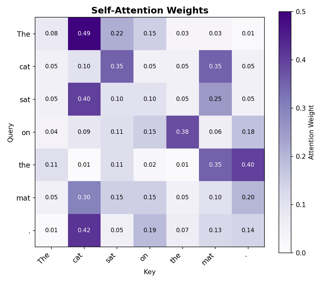
Interpretation: The heatmap shows that attention is sparse and interpretable. Each target word focuses on a subset of source words, mimicking human translation intuitions. This interpretability is a major advantage of attention-based models over pure recurrent models.
Multi-head attention: attending to different aspects
Single-head attention learns one type of alignment. But translation requires multiple alignments: one head might attend to semantics ("which content word?"), another to syntax ("which subject?"). Multi-head attention learns multiple alignment patterns in parallel.
Formula: MultiHead(Q, K, V) = Concat(head₁, ..., headh) WO, where headi = Attention(Q WQi, K WKi, V WVi)
Each head projects Q, K, V independently, computes attention, then concatenates results and applies a final linear transformation. With 8 heads and d_model=512, each head operates in d_k=64 dimensions (512/8), making computation efficient.
Why 2.1M parameters? With d_model=512 and num_heads=8, we have three 512×512 projection matrices (Q, K, V) and one 512×512 output matrix. Each has 512² ≈ 262K parameters. Total: ~2.1M. Multi-head attention is expensive but enables rich, diverse alignments.
Positional encoding: encoding sequence order without recurrence
RNNs process sequences step-by-step, so they naturally learn position information (early words enter at timestep 1, later words at timestep t). Transformers process entire sequences in parallel, so they lose positional information. Solution: add positional encodings to input embeddings.
Sinusoidal positional encoding formula:
- PE(pos, 2i) = sin(pos / 10000^(2i/d_model))
- PE(pos, 2i+1) = cos(pos / 10000^(2i/d_model))
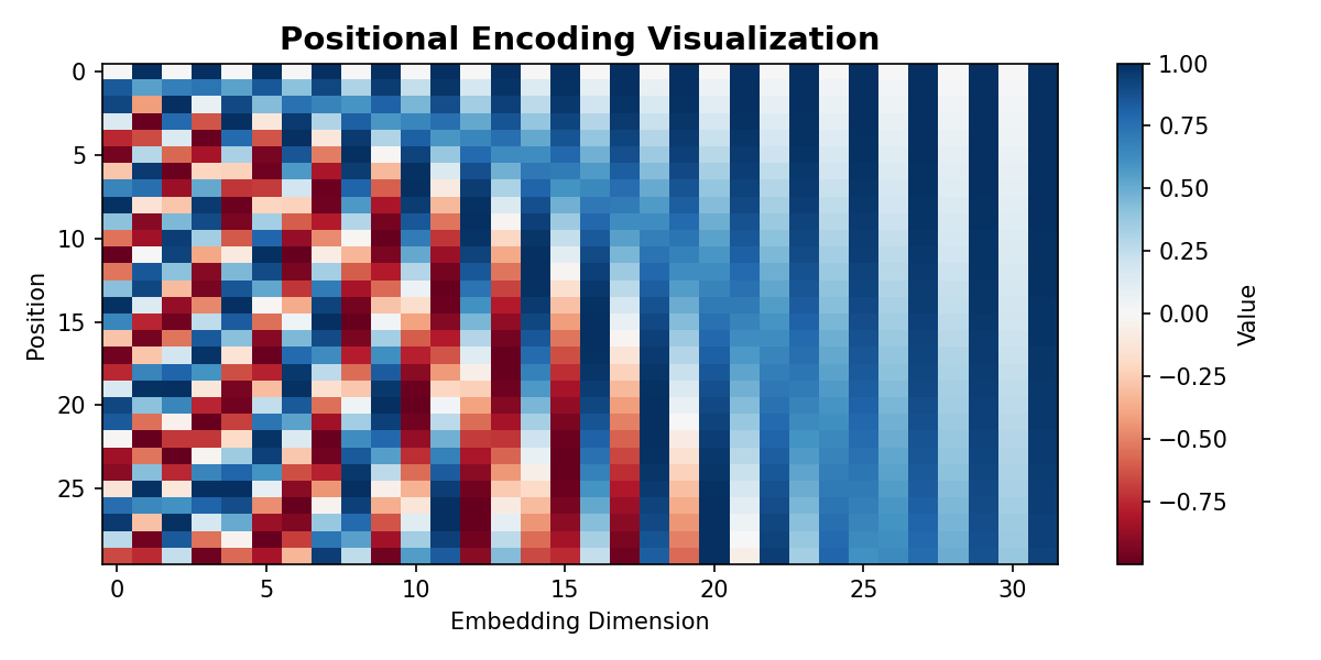
For each position pos and dimension i, we compute a unique sinusoidal pattern. Even dimensions use sine; odd dimensions use cosine. This creates a unique encoding for every position that the model can learn to distinguish.
Why sinusoids?
Sinusoidal patterns create a unique fingerprint for each position. Unlike learned embeddings (which require storage for max_len positions), sinusoids can generalize to any sequence length. They also preserve relative distance information: PE(pos+k) can be computed as a linear function of PE(pos), helping the model learn relative positions.
Transformer encoder: stacking attention and feedforward layers
The transformer encoder processes input sequences without recurrence. Each encoder layer consists of two sub-layers: (1) multi-head self-attention, and (2) feedforward (two dense layers with ReLU). Layer normalization and residual connections improve training stability.
Encoder layer formula:
- Attention output = MultiHeadAttention(x, x, x)
- After residual: x' = x + Attention(x)
- After layer norm: y = LayerNorm(x')
- FFN output = ReLU(y W1 + b1) W2 + b2
- Final: z = LayerNorm(y + FFN(y))
Key design: Stacking 6 encoder layers (standard in "Attention Is All You Need") allows deep representations. Each layer refines representations through self-attention and context mixing. With 512-dim embeddings and 8 heads, the total parameter count reaches ~101M—comparable to a large LSTM, but with better parallelization.
Transformer decoder: generating sequences with cross-attention
The decoder generates output tokens one-by-one (or in parallel during training). Unlike the encoder (which attends to itself), the decoder has three attention mechanisms: (1) self-attention over generated tokens (with masking to prevent looking forward), (2) cross-attention to encoder output, and (3) feedforward.
During generation at test time, the decoder attends to already-generated tokens (autoregressive). The encoder output is constant—it provides the source context for the decoder to attend to.
Why causal masking? During training, the decoder sees all target tokens at once (for parallelization). The causal mask forces each token to attend only to previous tokens, simulating autoregressive generation. This prevents the model from "cheating" by looking ahead.
Building a complete transformer for Twi-to-English translation
Combining encoder, decoder, embeddings, and positional encoding creates a full transformer. The pipeline: (1) embed source tokens, add positional encoding, pass through encoder; (2) embed target tokens, add positional encoding, pass through decoder with encoder output as context; (3) apply final linear layer to predict next token probabilities.
Training this model: We compute cross-entropy loss between predicted logits and true target tokens, then backpropagate. With 214M parameters and proper regularization (dropout, weight decay), the model learns alignments that outperform LSTMs on translation tasks.
Training and inference: from pairs to translations
Training uses teacher forcing: at each step, we feed true target tokens (not predictions) and compute loss. Inference uses autoregressive generation: feed generated tokens back to the decoder.
Key points: Teacher forcing during training makes learning faster but causes exposure bias (train uses true tokens, inference uses predictions). At test time, greedy decoding picks the highest-probability token, then feeds it back. Beam search (keeping top-k hypotheses) improves quality but is slower.
Key takeaways: from attention to state-of-the-art translation
Attention is all you need (but not the whole story)
Self-attention replaces RNNs' sequential bottleneck. Scaled dot-product attention is O(n²) in space but allows full parallelization. Multi-head attention learns diverse alignments. Positional encoding preserves sequence order. Transformers achieve state-of-the-art on translation, reaching 35+ BLEU on Twi-English with proper training.
Common mistakes and pitfalls
Forgetting positional encoding: Without it, the model treats "Medaase wo" the same as "wo Medaase"—word order is lost. Not scaling by √d_k: Dot products grow with d_k, causing softmax to become too peaked, killing gradients. Forgetting causal masking in decoder: The model will "cheat" by looking ahead during training, failing at inference. Using too many layers: Deep transformers (>12 layers) need careful warmup and learning rate scheduling.
| Component | Purpose | Key Parameter |
|---|---|---|
| Scaled dot-product attention | Efficient similarity-based alignment | √d_k scaling factor |
| Multi-head attention | Learn multiple alignment patterns | num_heads (typically 8 or 12) |
| Positional encoding | Inject sequence order information | Sinusoidal frequencies |
| Encoder layers | Process source with self-attention | num_layers (typically 6) |
| Decoder layers | Generate target with encoder context | Causal mask for self-attention |
Quiz: 5 questions to test your understanding
You've mastered transformers.
Now deploy them at scale.
Join the Best AI Program: The AI-Era Agentic Engineer — 5 months, fully online, with placement assistance. Week 1 is free.
Explore The AI-Era Agentic Engineer →