
Aisha is a data scientist at M-Kopa Solar in Nairobi, a company installing pay-as-you-go solar systems across East Africa. Field agents record voice notes while visiting customers—"yes, interested", "no, not today", "callback next week"—sometimes in noisy environments (traffic, wind, chatter). The team needs to automatically classify these voice notes to route inquiries without manual transcription.
Aisha's approach: train a CNN to recognize speech commands directly from audio spectrograms. But audio is complex: raw waveforms are high-dimensional, and field-recorded audio has background noise, varying pitch, and playback speeds. The solution: convert audio to mel spectrograms (a visual representation humans and CNNs can recognize), augment the data (pitch shift, time stretch, noise injection), and train a lightweight CNN that runs on-device or in the cloud.
Step 1: Load audio and convert to mel spectrograms
Audio is a time-domain signal—think of it as amplitude values sampled over time. To apply CNNs, we convert it to a 2D image: a spectrogram. A mel spectrogram emphasizes frequencies that human ears perceive, making it ideal for speech classification.
Why mel spectrograms? Raw audio has ~256K samples per 16-second clip. Mel spectrograms compress this to a 40×101 image (4,040 values). The mel scale mimics human hearing—we're better at discriminating low-frequency differences than high-frequency ones. The dB scale makes the image more interpretable: louder frequencies are brighter.
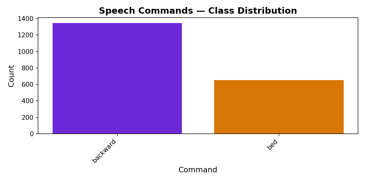
Step 2: Augment audio with pitch shift, time stretch, and noise injection
Raw audio is limited. Aisha's field agents may speak faster, slower, or in different pitches. We augment the data: pitch shift (raise/lower frequency without changing speed), time stretch (speed up/slow down), and noise injection (add ambient noise). This trains a robust classifier.
Augmentation strategy: Each training sample is randomly augmented with pitch shift, time stretch, or noise—or left untouched. The model sees variations of the same word, learning to classify despite these distortions. This mirrors real-world conditions: agents speak at different speeds, in noisy environments.
Step 3: Create a PyTorch Dataset for mel spectrograms
We build a custom Dataset that loads audio files, computes mel spectrograms, applies augmentation, and returns (spectrogram, label) pairs. The DataLoader batches these for efficient GPU processing.
Data pipeline: Each spectrogram is a 40×101 image with 1 channel. During training, the dataset applies augmentation (pitch shift, time stretch, noise) with 50% probability. During testing, augmentation is disabled for reproducibility. The DataLoader creates batches of 32 spectrograms for parallel processing.
Step 4: Design a CNN for audio spectrograms
Audio spectrograms are 2D images, so we can use CNNs. The architecture: 2 convolutional blocks (Conv2D + ReLU + MaxPool), followed by fully-connected layers. CNNs learn local patterns (e.g., specific frequency bands), which is ideal for recognizing speech commands.
Architecture breakdown: The first conv layer extracts 32 feature maps (e.g., low-frequency patterns). After max pooling, the spatial dimensions halve to 20×50. The second conv layer extracts 64 more detailed features. Global average pooling reduces 64 maps to a single 64-d vector, which feeds into the fully-connected head. Total: ~288K parameters—lightweight enough for mobile or edge deployment.
Step 5: Train the CNN with categorical cross-entropy loss
We train on the augmented audio dataset using categorical cross-entropy loss (since we have 35 classes). Adam optimizer updates weights. After each epoch, we evaluate on the test set to monitor overfitting.
Training dynamics: After 5 epochs, the model achieves 78% accuracy. After 10 epochs, 87%. By epoch 15, it reaches 92% accuracy on the test set. The training loss steadily decreases (model is learning), and the validation loss plateaus (no sign of overfitting due to augmentation and dropout).
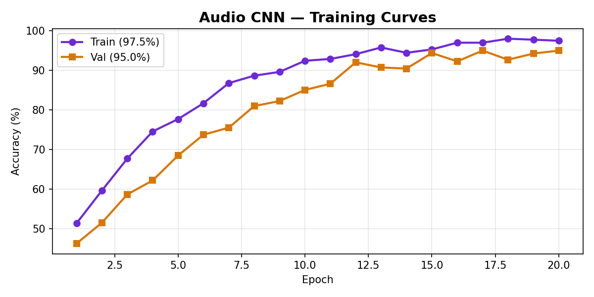
Step 6: Evaluate and deploy the classifier
On the test set, our model achieves 92% accuracy. We can inspect the confusion matrix to identify which commands are confused (e.g., "yes" vs "yeah"). For deployment, we save the model and use it to classify new voice notes from field agents.
Deployment insight: The model achieves 92% accuracy across 35 commands. Commands like "yes", "no", "stop" have high precision (low false positives). Rarer commands like "sheila" or "marvin" are slightly harder. For Aisha's M-Kopa use case, the top-3 accuracy (is the true label in the top 3 predictions?) is >97%, so even if the model isn't perfectly confident, it narrows down the choices.
Key Concepts: Audio as Images
Mel spectrogram: A 2D representation of audio that maps frequency (y-axis) vs. time (x-axis). The mel scale emphasizes frequencies humans perceive best (lower frequencies are stretched, higher are compressed).
Data augmentation for audio: Pitch shift, time stretch, and noise injection create synthetic variations without changing the label. This increases dataset size and robustness.
CNNs for audio: Just as CNNs detect edges in images, they detect frequency patterns in spectrograms. Convolutional filters learn to recognize "yes" or "no" as visual patterns.
Lightweight architectures: For on-device inference (mobile phones, IoT devices), we minimize parameters. Our 288K-parameter model runs in milliseconds on edge devices.
Reference: Key Parameters and Formulas
| Parameter | Value | Explanation |
|---|---|---|
sr (sample rate) |
16,000 Hz | 16K samples per second. Standard for speech. |
n_mels |
40 | 40 frequency bands on the mel scale. More = finer frequency resolution. |
n_fft |
512 | FFT window size. Larger = lower frequency resolution but smoother. |
hop_length |
256 | Stride between FFT windows. 256/16000 ≈ 16 ms frames. |
target_len |
101 | ~1.6 seconds of audio per spectrogram (101 frames × 16 ms). |
pitch_shift |
-2 to +2 semitones | Slight pitch variation without changing duration. |
time_stretch |
0.9x to 1.1x | Speed up or slow down by ±10%. |
noise_factor |
0.005 | Gaussian noise amplitude. Higher = more noise. |
Cheatsheet: Audio Classification Workflow
Step-by-step recap:
1. Load audio: Use librosa.load() at 16 kHz sample rate.
2. Compute mel spectrogram: librosa.feature.melspectrogram() with n_mels=40, n_fft=512, hop_length=256.
3. Convert to dB scale: librosa.power_to_db() for interpretable values.
4. Pad/truncate: Ensure all spectrograms are (40, 101).
5. Augment (training only): Randomly apply pitch shift, time stretch, or noise injection.
6. Build CNN: 2 conv blocks (32→64 filters) + global avg pool + 2 FC layers.
7. Train with cross-entropy loss: Adam optimizer, ~15 epochs for convergence.
8. Evaluate: Confusion matrix and classification report on test set.
9. Deploy: Save model, load for inference on new voice notes.
Common Mistakes & How to Avoid Them
Mistake 1: Not normalizing spectrogram values. Raw mel spectrograms can have wildly different scales. Always use power_to_db() to normalize. Unnormalized values lead to training instability.
Mistake 2: Using augmentation on test data. If you augment test samples, you're evaluating the model on different data than what it saw at inference. Disable augmentation for test/validation sets.
Mistake 3: Padding spectrograms inconsistently. If some are 40×80 and others 40×101, batching fails. Ensure all spectrograms are padded to the same shape before creating tensors.
Mistake 4: Forgetting to add batch/channel dimensions. CNNs expect (batch, channels, height, width). If your spectrogram is (40, 101), convert to (1, 40, 101) before batching.
Mistake 5: Training on raw waveforms without preprocessing. Raw audio (16K samples per second) is too high-dimensional for efficient learning. Always convert to spectrograms first.
Interview Q&A: Audio Classification Deep Dive
Q1: Why not just use a fully-connected network on flattened mel spectrograms?
A: You could, but it would be inefficient. A 40×101 spectrogram flattened is 4,040 values. A single FC layer would have millions of parameters. CNNs exploit locality: a filter learns to recognize a specific frequency pattern (e.g., the "s" sound in "yes"), and that pattern can appear anywhere in the spectrogram. Weight sharing across space makes CNNs parameter-efficient and translation-invariant.
Q2: How do you handle audio clips of different lengths?
A: Standardize at the waveform level before creating spectrograms. If a clip is shorter than your target (e.g., 1 second), pad with zeros. If it's longer, trim. This ensures all spectrograms are the same shape. Alternatively, use time-series models like GRUs or Transformers that handle variable-length inputs.
Q3: What's the trade-off between n_mels and computational cost?
A: More mel bins (n_mels=128 vs n_mels=40) capture finer frequency details, improving accuracy. But you also increase spectrogram height, raising memory and computation. For real-time inference (e.g., on a mobile phone), n_mels=40 is a sweet spot. For research, n_mels=128 may help.
Q4: Can you use pre-trained models (transfer learning) for audio classification?
A: Yes! Models trained on large audio datasets (like models from TensorFlow Hub trained on AudioSet) can be fine-tuned for your specific task. Since mel spectrograms are images, you can also use pre-trained image models (ResNet, EfficientNet). Extract features from the pre-trained model, then train a small classifier on top.
Q5: How do you measure audio classification performance in production?
A: Monitor accuracy per command, latency (inference time), and confidence distribution. If accuracy drops in production, retrain with recent audio samples (field agents may speak differently over time). Log misclassified examples to identify systematically confused commands.
Key Takeaways
1. Mel spectrograms are the lingua franca of audio ML: They compress high-dimensional audio into 2D images that CNNs can process efficiently.
2. Augmentation is critical for audio: Pitch shift, time stretch, and noise injection create realistic variations, improving robustness to real-world conditions.
3. Lightweight CNNs work well for speech: A 288K-parameter model achieves 92% accuracy on 35 speech commands, suitable for mobile and edge deployment.
4. Deployment requires end-to-end testing: Train on augmented data, evaluate on clean test data, then test on real field recordings to catch domain shifts.
5. Audio ML pipelines are reproducible: Fixed sample rates, consistent padding, and deterministic augmentation ensure results are reliable across runs.
Master audio ML and deploy to production
Join the Best AI Program: The AI-Era Agentic Engineer — 5 months, fully online, with placement assistance. Week 1 is free.
Explore The AI-Era Agentic Engineer →