
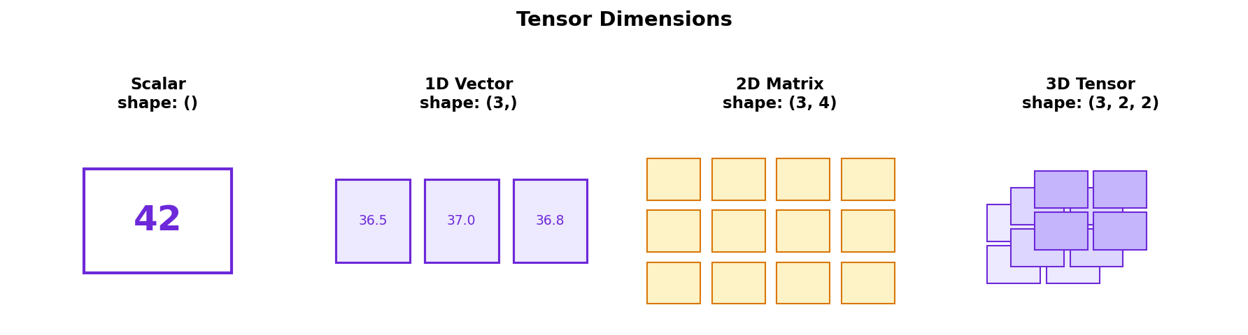
Arjun is an AI engineer at MedScan Diagnostics in Bangalore. He's building a CNN to detect lung abnormalities in X-ray scans. Each X-ray is a 224×224 grayscale image. When training, he processes 4 images at once in a batch. In PyTorch, this becomes a 4D tensor: [batch_size=4, channels=1, height=224, width=224]. Before building the neural network, Arjun must master tensor creation, indexing, reshaping, and PyTorch's killer feature—autograd.
Understanding tensors is the foundation. Without it, all the neural network code that follows is just magic. With it, you see exactly how data flows through every layer, how gradients propagate backward, and why GPU acceleration matters.
Creating tensors — from lists, zeros, randn, arange
PyTorch tensors are multi-dimensional arrays—the core data structure for neural networks. You can create them from Python lists, pre-allocate with zeros or random values, or generate sequences.
X-ray batch shape — the 4D medical imaging tensor
A batch of medical images in PyTorch follows the format: [batch_size, channels, height, width]. For Arjun's X-rays: 4 images, 1 channel (grayscale), 224×224 pixels = 4 × 1 × 224 × 224 = 200,704 elements total. This shape is crucial—neural networks expect exactly this layout.
Medical vitals matrix — indexing and selecting rows/columns
2D tensors represent tabular data. For MedScan patients: 3 patients, 4 vital signs (temp, heart rate, systolic BP, respiratory rate). NumPy-like indexing extracts rows, columns, or subsets.
Element-wise operations — add, multiply, broadcast
PyTorch tensors support element-wise arithmetic just like NumPy. Broadcasting automatically aligns shapes when possible—critical for neural network forward passes.
Dot product and matrix multiply — neural networks depend on these
Neural networks multiply data with weight matrices. The dot product (two vectors) and matrix multiplication (matrix × vector) are the core operations.
Reshape and view — rearrange dimensions without copying
view() reshapes without copying data (fast); reshape() handles non-contiguous tensors and may copy. For most cases, use reshape().
Squeeze and unsqueeze — add or remove dimensions
unsqueeze() adds a dimension of size 1; squeeze() removes them. Critical for matching tensor shapes in networks.
NumPy bridge — convert between NumPy and PyTorch
Data often starts in NumPy or pandas. PyTorch can convert without copying (shared memory)—modify one, the other updates too.
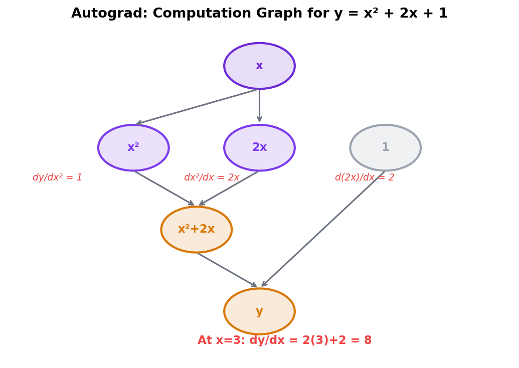
Autograd — automatic gradient computation (PyTorch's killer feature)
PyTorch computes gradients automatically. Set requires_grad=True on inputs, run forward pass, call .backward(), then access gradients via .grad. This is how neural networks learn.
How AI systems use this
Every pixel in an X-ray image, every vital sign in a patient record, every token in text—all become tensors. PyTorch operations on tensors are the language of neural networks. Forward passes multiply data with learned weights. Backward passes (via autograd) compute gradients that update those weights. CNNs apply convolution operations across 4D image tensors. RNNs step through sequence tensors. Transformers manipulate 3D token embeddings. Understanding tensors is understanding how AI models work at the lowest level.
Also used in...
Domain Spotlight
Task: Create a 4D tensor representing 8 X-ray images (224×224, 1 channel each). Add random noise to simulate real medical images, then extract the 5th image and reshape it to 1D for analysis.
Hint 1: xray_batch = torch.randn(8, 1, 224, 224)
Hint 2: Add noise: xray_batch += torch.randn_like(xray_batch) * 0.1
Hint 3: Extract 5th image: image_5 = xray_batch[4]
Hint 4: Flatten to 1D: image_1d = image_5.reshape(-1)
Expected shape: 1D tensor of 50,176 elements (224×224)
Interview questions: test your understanding
Quiz: 5 questions to test your knowledge
Cheatsheet: PyTorch tensor operations at a glance
| Operation | Syntax | Example |
|---|---|---|
| Create from list | torch.tensor([...]) |
torch.tensor([1, 2, 3]) |
| Zeros | torch.zeros((m, n)) |
torch.zeros((3, 4)) |
| Random normal | torch.randn((m, n)) |
torch.randn((5, 5)) |
| Arange | torch.arange(start, end, step) |
torch.arange(0, 10, 2) |
| Dot product | torch.dot(a, b) |
torch.dot(v1, v2) |
| Matrix multiply | A @ B |
W @ x |
| Reshape | tensor.reshape(shape) |
tensor.reshape(3, 4) |
| Unsqueeze | tensor.unsqueeze(dim) |
tensor.unsqueeze(0) |
| Squeeze | tensor.squeeze() |
tensor.squeeze() |
| NumPy bridge | torch.from_numpy(np_arr) |
torch.from_numpy(data) |
| Autograd | y.backward() |
loss.backward() |
Common mistakes: what breaks and how to fix it
requires_grad=True. Fix: x = torch.tensor([1.0], requires_grad=True).np_array = tensor.cpu().numpy() before NumPy ops.tensor = tensor + x instead of tensor += x during training.Key takeaways
Tensors are the foundation of deep learning. Master them, and neural networks become clear.
- Tensors are arrays: 0D scalars, 1D vectors, 2D matrices, 3D+ tensors. Images are 4D: [batch, channels, height, width].
- Shape matters: Operations depend on tensor dimensions. Always know your shapes. Use .shape and .numel().
- Broadcasting is powerful: PyTorch stretches dimensions automatically. Adding [64] bias to [1000, 64] data just works.
- Autograd is magic: Set requires_grad=True, run forward, call .backward(), access .grad. This is how networks learn.
- View vs reshape: view() is faster but requires contiguous tensors. reshape() is safer for general use.
- GPU acceleration: Same code, 10-100× speedup on GPU. Critical for large models.
You've mastered PyTorch tensors.
Now use them to build real neural networks.
Join the Best AI Program: The AI-Era Agentic Engineer — 5 months, fully online, with placement assistance. Week 1 is free.
Explore The AI-Era Agentic Engineer →