Master recurrent neural networks, vanishing gradients, LSTM gates, and sequence-to-sequence models. Process tonal languages and text sequences with PyTorch.
RNN • LSTM • GRU
Vanishing Gradients
Ghanaian NLP
22 min readIntermediate
🇬🇭
Meet Kwame
NLP Researcher Building Twi Language Tools
Kwame works on natural language processing for Ghanaian languages. He's building tools to process Twi—a tonal language where word order and subtle pitch changes carry meaning. CNNs treat pixels independently; for text, he needs models that understand sequences. RNNs process one word at a time, maintaining memory of what came before. But standard RNNs "forget" information over long sequences (vanishing gradients). LSTMs solve this with special gates.
1.2M
Twi words in corpus
8–12
Avg. words per sentence
1,000+
Unique tokens
📚 Why Sequences Matter
In image classification, each pixel is independent (mostly). In text, word order matters. The sentence "The dog bit the man" differs fundamentally from "The man bit the dog." RNNs are designed to process variable-length sequences, one timestep at a time, maintaining a hidden state that carries forward.
Sequences in Kwame's Twi Corpus
A Twi sentence like Ɔmom no dɔ aba (That woman came) is a sequence of 4 tokens. The model processes: [Ɔ] → [Ɔ, mɔm] → [Ɔ, mɔm, no] → [Ɔ, mɔm, no, dɔ] → [Ɔ, mɔm, no, dɔ, aba]. Each step outputs a prediction (next word, sentiment, POS tag). To predict "dɔ", the network needs memory of "Ɔ", "mɔm", "no".
🔄 Vanilla RNN: The Basics
A vanilla RNN has a hidden state h_t that updates at each timestep. At step t, it takes the current input x_t and the previous hidden state h_{t-1}, and produces a new hidden state h_t.
Vanilla RNN Forward Pass (Manual Implementation)
Vanilla RNN output
Output shape: torch.Size([8, 16, 1000])
This vanilla RNN works, but has a critical flaw: information from early timesteps (e.g., "Ɔ" at t=0) must be carried through 7 hidden state transformations to influence the output at t=7. Through repeated multiplications and tanh squashing, the gradient signal weakens exponentially—the vanishing gradient problem.
⚠️ The Vanishing Gradient Problem
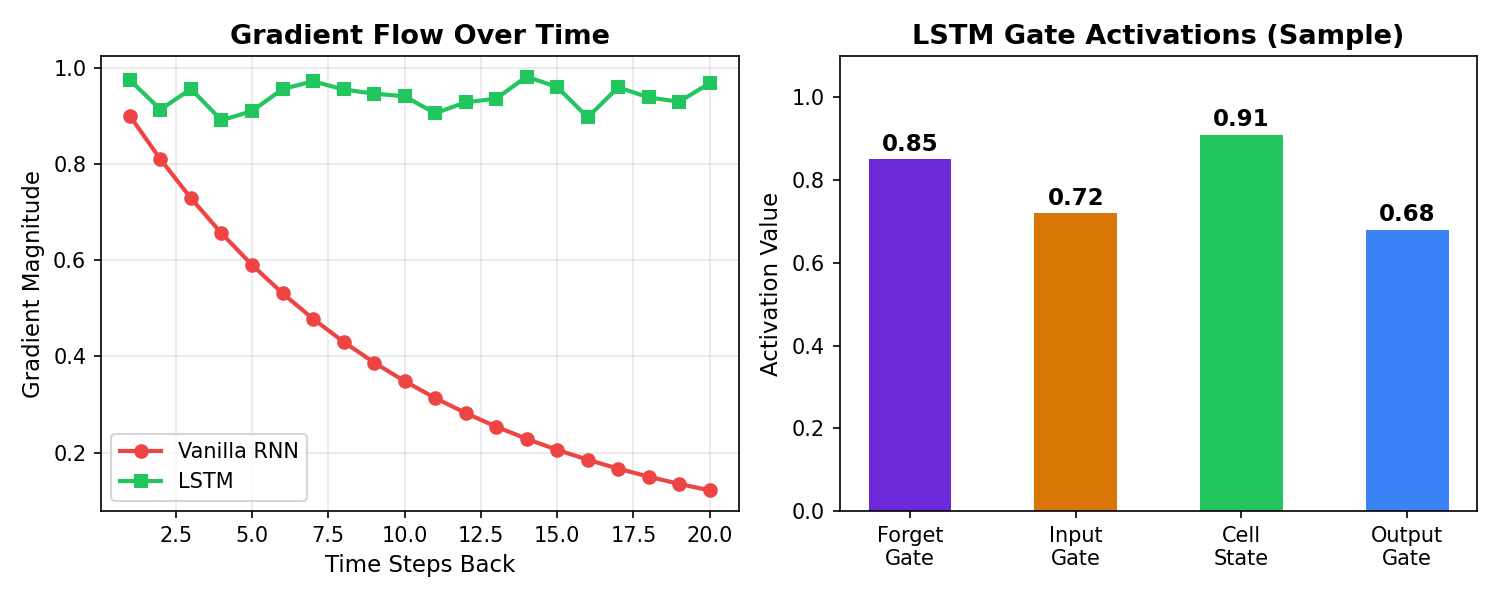
During backpropagation, gradients are computed via chain rule. In an RNN, the gradient at timestep 0 depends on multiplying gradients across 7 timesteps. If each multiplication is < 1 (typical for tanh, sigmoid), the product becomes exponentially small: 0.9^7 ≈ 0.48, but 0.1^7 ≈ 0.0000001.
Gradient magnitude vs timestep: vanilla RNN vs LSTM
The Problem
Early words in a Twi sentence (e.g., subject "Ɔ") are critical for understanding the whole sentence. But in a vanilla RNN, gradients from the loss at t=7 can't propagate back to t=0 effectively. The model learns long-range dependencies poorly.
The Solution: LSTM (Long Short-Term Memory)
LSTMs maintain a separate cell statec_t (memory) alongside the hidden state h_t. Three gates control what enters, leaves, and is forgotten: forget gate, input gate, and output gate. The cell state is updated by addition (not multiplication), so gradients flow unchanged—no vanishing.
🚪 LSTM Gates: Forget, Input, Output
An LSTM cell has four components: forget gate, input gate, candidate cell values, and output gate. Let's build intuition with Kwame's use case.
Forget gate (f_t): At "dɔ" (verb), forget old subject/tense info? Output ~0.1 (low). At "aba" (past marker), output ~0.95 (high—remember context).
Input gate (i_t): Does the new word matter? "dɔ" (critical verb) → i_t ≈ 0.8. Noise/filler words → i_t ≈ 0.2.
Output gate (o_t): Is it time to use memory? After punctuation/end-of-phrase → o_t ≈ 0.9. Mid-phrase → o_t ≈ 0.5.
⚡ GRU: Simplified LSTM
Gated Recurrent Unit (GRU) simplifies LSTM by merging forget and input gates into a single "reset gate" and combining cell state with hidden state. It has 2 gates instead of 3, trains faster, and often performs equally.
GRU is simpler (2 gates) and faster than LSTM (3 gates), but LSTM is more expressive. For long-range dependencies and very long sequences (>100 tokens), LSTM often wins. For typical Twi sentences (8-12 tokens), GRU is often sufficient and more efficient.
↔️ Bidirectional RNNs
A standard RNN reads left-to-right. Bidirectional RNNs read both left-to-right and right-to-left, then concatenate the two hidden states. For understanding Twi sentences, knowing future context (right) helps as much as past context (left).
Bidirectional LSTM for Twi POS Tagging
Bidirectional LSTM for sequence tagging
POS predictions shape: torch.Size([16, 8, 10])
Word "no" (prep/conj): forward context + backward context → accurate POS tag
When to Use Bidirectional
POS tagging, NER, Chunking: Label each word based on full sentence → bidirectional ✓
Language modeling, next-word prediction: Can't see future words → unidirectional (forward only)
Machine translation encoder: Encode full source sentence → bidirectional ✓
Machine translation decoder: Generate word by word → unidirectional (left-to-right)
🔄 Sequence-to-Sequence (Seq2Seq) Basics
Seq2Seq models encode a variable-length input sequence and decode it into a variable-length output sequence. Examples: Twi→English translation, summarization, Q&A.
Seq2Seq Encoder-Decoder with Attention (Simplified)
Seq2Seq encoder-decoder
Translation shape: torch.Size([16, 12, 1000])
Encoder processes: "Ɔ mɔm no dɔ aba"
Decoder generates: "The woman came long ago"
🏆 Mini Challenge: Compare RNN Architectures
Task: Build three models for Twi sentiment classification (positive/negative): (1) Vanilla RNN, (2) LSTM, (3) Bidirectional LSTM. Train each on 1,000 Twi sentences. Which achieves the best accuracy? Why?
Hint: Vanilla RNN will struggle on longer sentences due to vanishing gradients. LSTM should improve accuracy. Bidirectional LSTM can see future context, potentially capturing nuanced sentiment cues.
💼 Interview Questions
In vanilla RNNs, gradients are computed through repeated multiplications during backpropagation. Each multiplication is typically < 1 (due to tanh/sigmoid squashing), so gradients exponentially decay as they propagate backward through time. This means early timesteps receive almost no gradient signal, so the network can't learn long-range dependencies. For example, in an 8-word Twi sentence, the first word's impact on the loss is nearly zero by the 8th word.
Forget gate, input gate, and output gate. The forget gate decides what information to discard from the cell state. The input gate decides what new information to add. The output gate decides which part of the cell state to expose as the next hidden state. These gates are sigmoid outputs (0 or 1), so they act as soft switches controlling information flow.
LSTM maintains a cell state that is updated by addition: C_t = f_t * C_{t-1} + i_t * C_tilde. The multiplication f_t is just a gate value (0 to 1), not a repeated squashing function. Crucially, the '+' operation preserves gradient flow without multiplying through nonlinearities repeatedly. When computing gradients with respect to C_0 from C_t, the gradient simply backpropagates through additions and gates, not through stacked tanh functions. The gates modulate (multiply) the signal, but the cell state itself maintains an additive path.
Bidirectional RNNs see the entire sequence (past and future). Use bidirectional for tasks where the full context helps: POS tagging, named entity recognition, sentence classification. Use unidirectional (forward-only) for tasks where you can't peek ahead: language modeling, next-word prediction, streaming applications. In Twi POS tagging, bidirectional is better because the role of a word depends on surrounding words. In next-word prediction, unidirectional is necessary because the future doesn't exist yet.
Common issues: (1) Exposure bias—training with teacher forcing (always using ground truth), but inference uses predictions (errors compound). Fix: use scheduled sampling (mix ground truth and predictions during training). (2) No attention—the decoder ignores encoder outputs and relies only on the final hidden state, losing source information. Fix: add attention mechanism (let decoder focus on different encoder timesteps for each output). (3) Length mismatch—decoder doesn't know when to stop. Fix: use an token and train to predict it. (4) Poor initialization—encoder and decoder hidden sizes don't match. Fix: ensure consistency or use projection layers. (5) Insufficient training data—need thousands of parallel (Twi, English) sentence pairs. Fix: use transfer learning or back-translation to augment data.
✓ Quick Quiz
Question 1 / 5
In a vanilla RNN processing an 8-word Twi sentence, the first word's gradient signal degrades as it backpropagates through 7 timesteps. Why?
Question 2 / 5
An LSTM cell has a forget gate that outputs 0.8 and an input gate that outputs 0.6. What fraction of the cell state is updated with new information?
Question 3 / 5
You're building a bidirectional LSTM for Twi POS tagging. How many hidden states does the forward LSTM produce?
Question 4 / 5
GRU vs LSTM: which is typically faster and why?
Question 5 / 5
In seq2seq Twi→English translation, the encoder outputs 8 hidden states (one per Twi word). The decoder needs to generate 12 English words. How does the decoder use encoder information?
Twi sentences vary in length (4-15 words). If you pad all to 20 words and feed to LSTM, the model wastes computation on padding tokens. Use pack_padded_sequence and pad_packed_sequence to skip padding during LSTM computation. This significantly speeds up training.
Using only the final hidden state for classification
For sentence classification (sentiment, intent), using only h_n makes sense. For POS tagging or NER, you need predictions for every word, not just the last. Use the full output sequence from LSTM and apply a classifier at each timestep.
Mismatching batch_first and tensor shapes
PyTorch LSTM expects (seq_len, batch, input_size) by default. If you set batch_first=True, it expects (batch, seq_len, input_size). Always check your input shape. Common error: x.shape = (16, 128, 8) interpreted as (16 tokens, 128 features) instead of (16 batches, 128 tokens, 8 features).
Bidirectional RNN in autoregressive tasks
You cannot use bidirectional RNN for next-word prediction—the model would see future words, which is cheating. Bidirectional only works for non-autoregressive tasks (tagging, encoding). For language models, use forward-only unidirectional RNN.
Seq2seq without handling variable-length outputs
Your encoder always outputs length 8 (Twi sentence), but the decoder must generate variable-length English (sometimes 10, sometimes 15 words). Either fix output length (bad) or use an token and teach the decoder to emit it when done (good). Or use attention to let the decoder focus on source words dynamically.
✦ Key Takeaways
RNNs process sequences one timestep at a time, maintaining a hidden state. Vanilla RNNs suffer from vanishing gradients—gradients decay exponentially as they backpropagate through time.
LSTMs solve vanishing gradients by maintaining a cell state updated by addition (not multiplication), plus three gates (forget, input, output) that control information flow. This allows gradients to flow unchanged over long sequences.
GRU is a simplified LSTM with 2 gates instead of 3—typically 10-20% faster with similar accuracy. Use GRU for efficiency; use LSTM for expressiveness on very long sequences.
Bidirectional RNNs see the full sequence (left and right context). Use for tagging and classification. Use unidirectional (forward-only) for language modeling and streaming applications where the future is unknowable.
Seq2seq encodes a source sequence (Twi) and decodes it into a target sequence (English). Basic seq2seq uses the encoder's final hidden state; more advanced versions use attention to let the decoder focus on different source words for each output.
Kwame's Twi→English NLP system relies on LSTMs to capture long-range grammatical and semantic dependencies in tonal languages where word order and pitch are critical.