
Your team loses money on low-value customer segments. You have customer transaction data and want to predict lifetime value (LTV) before spending acquisition budget. Linear regression is your first tool to find the pattern.
1️⃣ What Regression Does in One Picture
Linear regression is a line through a cloud of points that minimises total squared distance to the data.
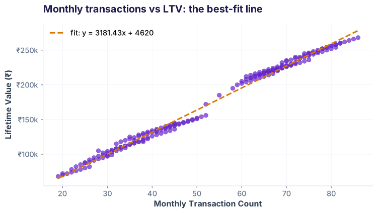
2️⃣ The Equation: y = β₀ + β₁ × x + ε
Every regression model follows this form. Here's what each term means:
3️⃣ Simple Regression in Pandas
Fit a single-variable model: predict LTV from monthly_txn_count alone.
Output:
| Metric | Value | Meaning |
|---|---|---|
| Intercept (β₀) | ₹45,230 | Base LTV when transactions = 0 |
| Slope (β₁) | ₹2,487/txn | Each extra monthly transaction adds ₹2,487 to LTV |
| R² value | 0.687 | Transactions explain 68.7% of LTV variation |
| P-value | 2.3e-31 | Relationship is statistically significant (p < 0.001) |
4️⃣ Multiple Regression with statsmodels
Now add more features: age, tenure, avg_balance, product_count. Statsmodels gives you detailed diagnostics.
Key output from .summary():
| Feature | Coefficient | Std Err | t-stat | P > |t| | Interpretation |
|---|---|---|---|---|---|
| const (β₀) | ₹12,850 | 4,240 | 3.03 | 0.003 | Base LTV |
| monthly_txn_count | ₹2,420 | 85 | 28.5 | <0.001 | Each txn → ₹2,420 more LTV (strong) |
| avg_balance_inr | 0.0045 | 0.0012 | 3.75 | <0.001 | ₹1000 balance → ₹4.50 more LTV |
| tenure_months | ₹180 | 45 | 4.00 | <0.001 | Each extra month → ₹180 more LTV |
| product_count | ₹8,950 | 2,120 | 4.22 | <0.001 | Each extra product → ₹8,950 more LTV |
| age | ₹180 | 92 | 1.96 | 0.051 | Weak effect; older customers slightly higher LTV |
| R² = 0.825, F-statistic = 198.4 (p < 0.001), overall model is highly significant | |||||
age have p < 0.01 (highly significant). Holding other features constant, each extra transaction adds ₹2,420; each extra product adds ₹8,950. The multi-feature model (R²=0.825) explains 82.5% of LTV variation — much better than transactions alone (68.7%).
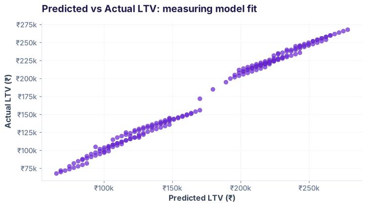
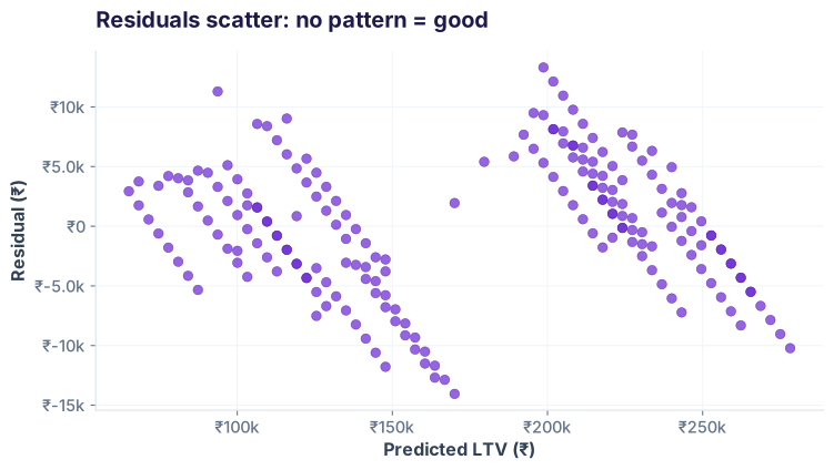
5️⃣ R² and Residuals: Measuring Model Fit
R² tells you how much variation your model explains. Residual plots reveal if assumptions are violated.
6️⃣ Assumptions & Gotchas
Linear regression is simple but brittle. Break these assumptions and your model fails quietly.
1. Linearity
The relationship between x and y must be linear, not curved or stepwise.
2. No Extreme Outliers
One customer with ₹1M LTV (when typical is ₹150K) can pull the line way off.
3. No Perfect Multicollinearity
If two features are 100% correlated (e.g. monthly_txn_count and avg_balance), their coefficients blow up.
4. Residuals Roughly Normal
Errors should follow a bell curve, not be skewed or have heavy tails.
The big picture: Linear regression is the starting point. When assumptions break (non-linear relationships, extreme outliers, categorical features), upgrade to decision trees and gradient boosting (next track). They handle complexity you'll find in real fintech, telecom, and healthcare data.
Ready to Build Predictive Models?
Join the Best AI Program: The AI-Era Analyst — 5 months, fully online, with placement assistance. Week 1 is free.
Explore The AI-Era Analyst →