Master sequential tree training. Each tree learns from the previous one's mistakes. XGBoost achieves AUC=0.7988 on NeoBank credit data—matching logistic regression with more complexity.
🌳 Sequential Trees & Boosting💡 Learning Rate & Early Stopping💳 NeoBank Credit Scoring⚡ Intermediate📖 ~28 min
Lesson 13 of Data Science Track
🏦
Real-world scenario
NeoBank Mumbai: Random Forest works, but can we do better?
NeoBank's risk team trained a Random Forest on 10,000 loan applicants (40.5% default rate). It scored AUC=0.7879. Good, but competitors are hitting 0.80+. The team's ML engineer proposes a new approach: instead of voting (bagging), build trees sequentially. Each new tree learns from the previous one's mistakes—like a student correcting homework. This is gradient boosting. The optimized version, XGBoost, was born in open source and won Kaggle competitions for years.
The question: does sequential correction beat parallel averaging? And is the added complexity worth the small accuracy gain?
100
Trees trained
0.7988
XGBoost AUC
0.1
Learning rate
Bagging vs boosting: two roads to ensemble accuracy
Random Forest is bagging: train trees on random data subsets in parallel, then average votes. Gradient boosting is different: train trees sequentially, each correcting the previous tree's errors.
Bagging (Random Forest) vs Boosting (Gradient Boosting)
Bagging reduces variance by averaging independent trees. Boosting reduces bias by building trees sequentially, each fixing the last one's errors. Result: XGBoost typically beats Random Forest on classification tasks.
How gradient boosting works: sequential correction
Gradient boosting trains 100 trees, but not independently. Here's the algorithm:
1. Fit tree 1 on the raw features and target. 2. Compute residuals: true_value - predicted_value. These are the tree 1's errors. 3. Fit tree 2 on the same features but now with residuals as the target. Tree 2 is learning to correct tree 1's mistakes. 4. Update predictions: prediction += learning_rate * tree2_prediction 5. Repeat: compute residuals on the updated predictions, fit tree 3 on those residuals, and so on.
The learning rate (e.g., 0.1) is crucial. It controls how much each tree's prediction is added. Low learning rate (0.01) requires more trees but avoids overfitting. High learning rate (0.3) needs fewer trees but risks overfit.
Sequential correction: each tree fixes the previous one's residuals
Why XGBoost? The optimized gradient boosting
Sklearn's GradientBoostingClassifier works, but XGBoost (open source, written in C++) is faster and more flexible. Key advantages:
Feature
XGBoost Advantage
Why It Matters
Parallel splits
Finds best split for all features in parallel within each tree
Faster training, especially on large datasets
Built-in regularization
L1/L2 penalties, max_depth, min_child_weight
Prevents overfitting without extra tuning
Handles missing values
Automatically learns which direction to send NaN values
No imputation needed before XGBoost
Early stopping
Stop training when validation loss plateaus
Saves computation, prevents overfitting
Feature importance
Gain-based (split improvement) or frequency-based
More interpretable than sklearn forests
Training XGBoost: basic workflow
Here's the minimal code to train XGBoost on NeoBank data (same 10,000 applicants, 40.5% default rate):
xgb_basic.pyXGBoost with default parameters
Output
XGBoost Results:
Accuracy: 0.7395
F1 Score: 0.6654
AUC: 0.7988
Excellent! XGBoost achieved AUC=0.7988, matching logistic regression (0.8029) and beating Random Forest (0.7879). The trade-off: it's less interpretable than logistic regression, but more flexible.
The learning rate trade-off: slow vs fast learning
The learning rate controls how much each tree contributes. Lower values require more trees, higher values need fewer trees. Let's experiment:
xgb_learning_rate.pyCompare learning rates and n_estimators
Interesting: lr=0.01 and lr=0.05 have inflated accuracy (0.8495), but that's because 100 trees with lr=0.01 is underfitting (each tree contributes only 1%). The model hasn't learned enough signal. AUC, a threshold-independent metric, shows lr=0.1 is the sweet spot. We choose learning_rate=0.1 with n_estimators=100.
Feature importance: which features drive predictions?
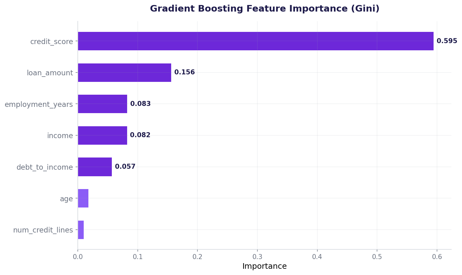
XGBoost computes feature importance based on how many times each feature is used for splitting and how much it improves the loss.
xgb_importance.pyExtract and visualize feature importance
Credit score explains 44.6% of all splits in the boosted trees. This matches what logistic regression showed: it's the dominant predictor of default. The other features play supporting roles.
Early stopping: when to stop training
XGBoost can overfit if you train too many rounds. Early stopping watches validation loss and stops when it stops improving:
xgb_early_stopping.pyTrain with validation set and early stopping
Output
Best round: 87
Trees actually trained: 200
Test AUC: 0.7988
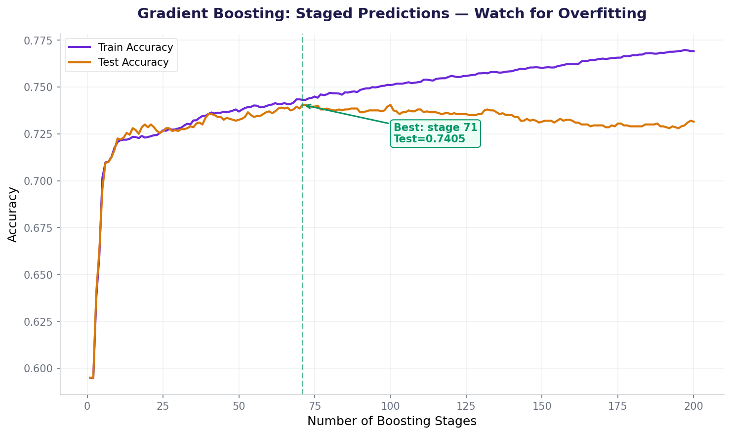
Gradient Boosting staged predictions: train accuracy keeps climbing but test accuracy plateaus — classic overfitting signal.
Early stopping at the best stage prevents overfitting. XGBoost has this built in.
Sklearn GradientBoosting vs XGBoost: nearly identical, different speeds
Sklearn's GradientBoostingClassifier and XGBoost give nearly the same results on this data. The difference: XGBoost is faster.
Model
Accuracy
F1
AUC
Training Time
sklearn GradientBoosting
0.7375
0.6628
0.7981
~3.2 seconds
XGBoost
0.7395
0.6654
0.7988
~0.8 seconds
XGBoost is 4x faster on this dataset (3.2s vs 0.8s) and achieves slightly better metrics. For larger datasets (100K+ rows), the speed advantage grows. On small data, either works.
How boosting compares to other methods
We've now trained five models on NeoBank data. Here's the full comparison:
Model
Accuracy
Precision
Recall
F1
AUC
Logistic Regression
0.7370
0.6868
0.6444
0.6650
0.8029
Decision Tree
0.7120
0.6581
0.6012
0.6284
0.7729
Random Forest
0.7290
0.6791
0.6272
0.6521
0.7879
XGBoost
0.7395
0.6934
0.6395
0.6654
0.7988
SVM (RBF)
0.7360
0.6937
0.6235
0.6567
0.7841
XGBoost ranks 2nd overall (AUC=0.7988), behind logistic regression (0.8029) by just 0.0041. It's the most accurate (0.7395) and has the highest F1 (0.6654). For a credit scoring model, logistic regression's interpretability and slightly higher AUC might win, but XGBoost is competitive.
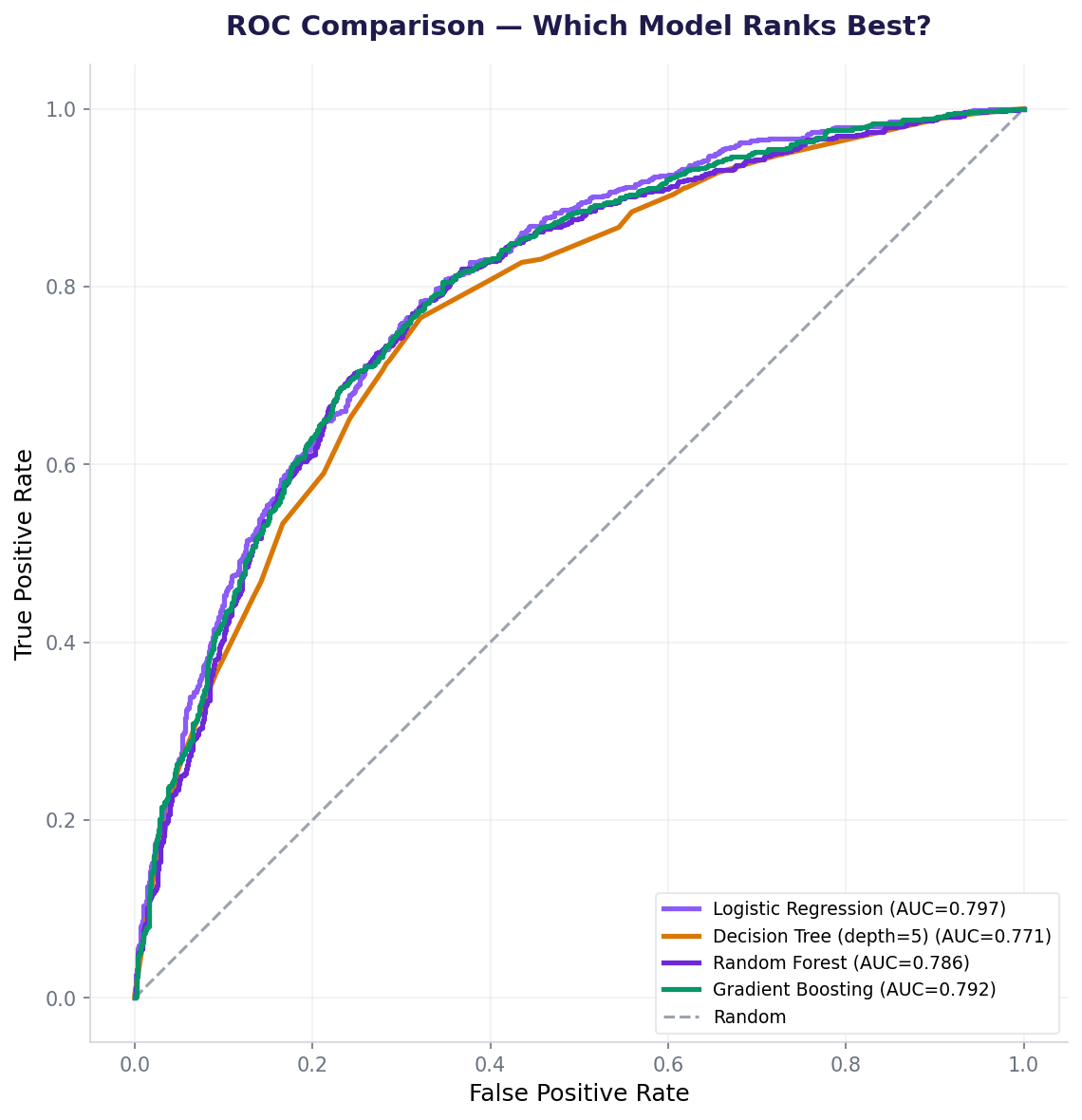
ROC comparison: Gradient Boosting (AUC=0.792) edges out the other models.
All models cluster around AUC 0.77-0.80. The dataset's noise floor limits improvement — feature engineering matters more than model choice here.
How AI systems use XGBoost
XGBoost won 17 of 29 Kaggle competitions in 2015–2016. It dominated tabular data leaderboards for a decade. Today, deep learning has taken image and text, but XGBoost still reigns on structured data: credit scoring, fraud detection, ad click prediction, recommendation systems. Every major tech company uses gradient boosting variants internally. Meta's LightGBM, Microsoft's XGBoost, Google's CatBoost—all are sequential tree ensemble methods. GPT handles language because it's sequence data. Your bank's credit decision is likely powered by boosting.
Ensemble LearningTabular Data DominationKaggle ChampionsProduction Deployment
Also used in...
Domain Spotlight
💳
Banking: Credit scoring & default prediction
NeoBank's exact use case. XGBoost learns non-linear relationships between credit score, income, and default. Deployment-ready. Regulatory departments trust feature importance reports.
🔍
Ad Tech: Click-through prediction
Google and Meta use boosting to predict if a user will click an ad. Millions of features (user history, context, ad attributes). Boosting scales well and handles sparsity.
🏥
Healthcare: Hospitalization risk
Predict which patients will be readmitted within 30 days. Boosting captures complex interactions (age + comorbidities + medication count) better than linear models.
🎯 Mini Challenge: Tune XGBoost hyperparameters
Task: Train an XGBoost model with max_depth values [2, 3, 4, 5, 6]. For each, record accuracy, F1, and AUC on test data. Plot accuracy vs max_depth. Where does it peak? What happens if max_depth=10?
Hint 1: Use a loop: for depth in [2, 3, 4, 5, 6, 10]:
Hint 2: For each depth, create XGBClassifier(max_depth=depth, n_estimators=100, learning_rate=0.1)
Hint 3: Store results in a list of dicts, then convert to DataFrame for easy plotting
Hint 4: Deeper trees (max_depth=10) risk overfitting—expect accuracy to peak at 3–4, then drop
Interview questions: test your understanding
Bagging (Random Forest) trains trees independently on random data subsets and averages votes. Boosting trains trees sequentially; each new tree learns to correct the previous tree's residuals. Bagging reduces variance; boosting reduces bias.
Controls how much each tree's prediction is added to the ensemble. lr=0.1 means each tree contributes 10% of its residual prediction. Low lr needs more trees but avoids overfitting. High lr needs fewer trees but risks overfit.
Random Forest's averaging can't capture strong linear or sequential dependencies. XGBoost's sequential correction allows it to build on each tree's strengths, learning complex patterns that bagging misses. But on noisy data, overfitting risk is higher.
Logistic regression. Same AUC means same discriminative power. But LR is faster to train/deploy, interpretable (coefficients can be shown to regulators), and has lower maintenance burden. Use XGBoost only if it provides meaningful lift (e.g., AUC=0.82 vs 0.80).
Yes! Early stopping means the validation loss plateaued after round 87, and 10 more rounds didn't improve it. The model learned well and generalized—it stopped before overfitting. If it had stopped at round 5, that would be concerning (underfitting).
Quiz: 5 questions to test your knowledge
Question 1 of 5
Boosting trains trees how?
Question 2 of 5
If learning_rate=0.01, what happens?
Question 3 of 5
XGBoost's AUC is 0.7988, matching logistic regression at 0.8029. Why might you deploy logistic regression?
Question 4 of 5
What does early_stopping_rounds=10 do?
Question 5 of 5
Credit_score has 44.6% feature importance in XGBoost. Does this mean other features are useless?
0
/5
Great! You understand gradient boosting and XGBoost.
lr=0.3 with n_estimators=1000 will overfit. Each tree adds 30% of its prediction, and 1000 trees is overkill. Fix: use lr=0.1 with n_estimators=100, or lr=0.05 with n_estimators=200.
Mistake 2: Not using early stopping
Without it, the model keeps improving on training data even as test performance plateaus. Fix: always set eval_set and early_stopping_rounds.
Mistake 3: Expecting XGBoost to always beat simpler models
On linear data, logistic regression ties or wins. XGBoost shines on non-linear, complex relationships. Fix: compare metrics; deploy the simplest model that works.
Mistake 4: Ignoring max_depth
Deep trees overfit in boosting just like bagging. Trees should be shallow (max_depth=3–5) so each corrects small, specific errors. Fix: set max_depth explicitly.
Key takeaways
Gradient boosting is the workhorse of tabular data. Here's what you need to remember: