
NeoBank's risk team trained logistic regression and random forests. Both scored AUC=0.80. But they wonder: can we find a boundary that maximizes the gap between the two classes? A boundary with a wide margin tends to generalize better.
That's where Support Vector Machines come in. SVM finds the hyperplane (decision boundary) that leaves the maximum margin—the widest empty space—between the closest defaulters and non-defaulters. These closest points are called support vectors.
What is SVM? Finding the widest margin
In binary classification, you need a line (or hyperplane in high dimensions) that separates two classes. Infinite lines can do this. But which one is best?
Support Vector Machines pick the line with the widest gap—the largest margin—between the two classes. The intuition: a boundary with room to spare will handle new, slightly different data better than a tight boundary that just barely separates.
Support vectors: The data points that define the margin (the closest ones to the boundary).
Goal: Maximize the margin while keeping misclassifications low.
Support vectors: the decision makers
Most data points don't matter. Only the points closest to the boundary—the support vectors—influence the decision boundary. If you move a point far from the boundary, it won't change SVM's decision. But move a support vector, and the entire boundary shifts.
This is why SVM is efficient: once trained, you only need to store and evaluate the support vectors, not the entire dataset.
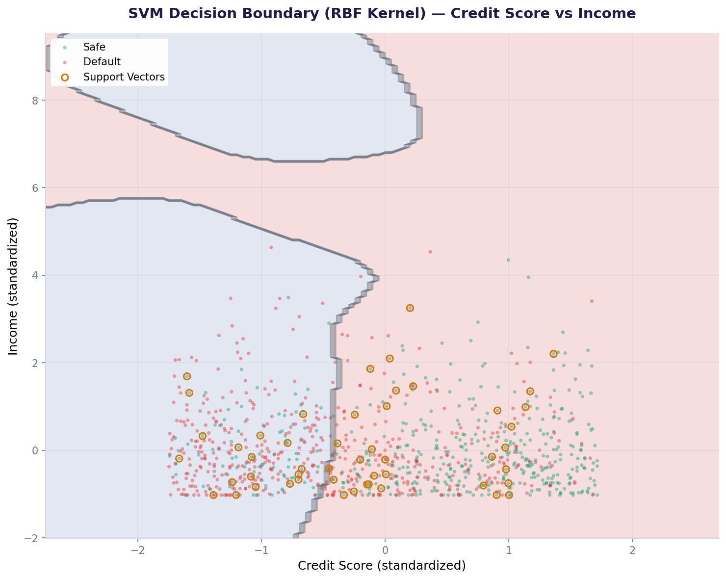
The kernel trick: non-linear boundaries
What if the data isn't linearly separable? In 2D, a single line can't separate the classes. But if we could add a third dimension, the points might separate with a plane.
The kernel trick does this implicitly. It transforms data to a higher-dimensional space without actually computing the transformation. Three kernels are common:
| Kernel | Boundary Type | When to Use | Code |
|---|---|---|---|
| Linear | Straight line / flat hyperplane | Data is (mostly) linearly separable | kernel='linear' |
| RBF (Radial Basis Function) | Curved, non-linear boundary | Non-linear relationships; default choice | kernel='rbf' |
| Polynomial | Polynomial curves (degree 2, 3, ...) | Non-linear but want interpretability | kernel='poly', degree=3 |
The kernel trick computes similarity between points instead of coordinates. For RBF: K(x, y) = exp(-gamma * ||x - y||²). Two points far apart have low similarity; nearby points have high similarity.
Training SVM with scikit-learn
Always scale features first. SVM computes distances; unscaled features distort the boundary. Use StandardScaler.
The C parameter: margin vs. misclassification trade-off
C controls the penalty for misclassifying a point. Low C allows more misclassifications for a wider margin (underfitting). High C penalizes misclassifications heavily, creating a narrow, complex boundary (overfitting).
Sweet spot: C=1.0 or C=10.0. Beyond C=100, test accuracy drops—overfitting. With C=0.1, the model underfits slightly.
Comparing kernels: linear vs. RBF vs. polynomial
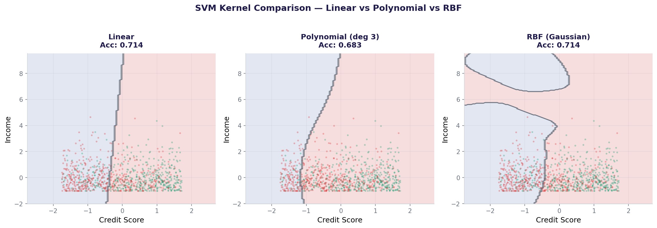
Different kernels create different decision boundaries. Let's train all three on the same data.
RBF wins on AUC. Linear is close and faster. Polynomial underperforms. For this dataset, the relationship is nearly linear, so RBF's complexity doesn't add much.
Why SVM requires scaling
SVM computes distances between points. Without scaling, features with large ranges dominate. Example: if credit_score ranges 300-850 and income_ratio ranges 0-1, the distance is almost entirely determined by credit_score.
Huge difference! Scaling boosts accuracy by 15 points. Always scale before SVM.
How SVM fits into modern AI
SVMs dominated machine learning before deep learning. They won competitions, powered spam filters, and detected faces in images. Today, deep neural networks outperform SVMs on images and text. But on tabular data (credit scoring, insurance, biology), SVMs remain competitive and interpretable. The kernel trick—implicitly mapping to higher dimensions—influenced how neural networks handle non-linearity.
Also used in...
Domain Spotlight
Task: Train SVM with RBF kernel using C values [0.01, 0.1, 1, 10, 100]. For each, print train accuracy, test accuracy, and number of support vectors. Which C minimizes test accuracy loss while keeping support vectors low?
Hint 1: Loop over c_values and train inside: for c in [0.01, 0.1, 1, 10, 100]:
Hint 2: Number of support vectors: len(svm.support_)
Hint 3: Test accuracy: svm.score(X_test_scaled, y_test)
Hint 4: Look for the "elbow point" where test accuracy is good but support vectors plateau.
Interview questions: test your understanding
Quiz: 5 questions to test your knowledge
Cheatsheet: SVM at a glance
| Concept | Code | Notes |
|---|---|---|
| Train SVM | SVC(kernel='rbf') |
Always scale first with StandardScaler |
| Linear kernel | kernel='linear' |
Fast, interpretable, for linear data |
| RBF kernel | kernel='rbf' |
Default, non-linear boundaries, slower |
| Polynomial kernel | kernel='poly', degree=3 |
Polynomial boundaries, tune degree |
| C parameter | C=1.0 |
Low C = wide margin; high C = narrow margin |
| Support vectors | svm.support_ |
Indices of training points defining boundary |
| Probabilities | probability=True, then predict_proba() |
SVM uses Platt scaling to calibrate probs |
Common mistakes: what breaks and how to fix it
StandardScaler().fit_transform(X_train) before fitting.Key takeaways
- SVM finds the widest margin between classes. Only support vectors (closest points) define the boundary.
- Always scale features first. SVM computes distances; unscaled features dominate.
- Kernel trick enables non-linear boundaries: RBF for non-linear data, linear for fast inference on linearly separable data.
- C parameter controls the margin-misclassification trade-off. Low C = wider margin, high C = narrow, complex boundary.
- SVM on tabular data is competitive, but slower on large datasets than logistic regression or boosting.
- When AUC is tied with simpler models, choose simplicity: logistic regression is faster and more interpretable.
Ready to deploy classification models?
Join the Best AI Program: The AI-Era Analyst — 5 months, fully online, with placement assistance. Week 1 is free.
Explore The AI-Era Analyst →