
You're a data scientist at NeoBank, a digital bank in Mumbai. The risk committee has trained 5 different classification models on 10,000 loan applicants. Each model works—but which one should the bank deploy?
Logistic Regression is fast and interpretable. Random Forest and XGBoost are "fancier"—do they earn their complexity? Decision Trees are transparent to regulators. SVM captures non-linear patterns. Today, you'll build all five, compare them side-by-side, and recommend one to the board. The answer isn't always "the most accurate."
The business brief: which model should NeoBank deploy?
Before we build, let's set the decision criteria. The CEO asks three questions:
2. How well does it rank applicants? — AUC (does it assign higher default probability to actual defaulters?).
3. Can we explain it? — Logistic Regression coefficients vs XGBoost's black box.
4. Is it fast enough? — Tree-based models are slower than logistic regression at inference.
5. Does it handle production updates? — How often do we retrain? What if defaults shift?
Phase 1: Exploratory data analysis
First, we explore the NeoBank credit dataset. 10,000 applicants, 11 columns. Let's spot the patterns that models will learn.
Key EDA findings
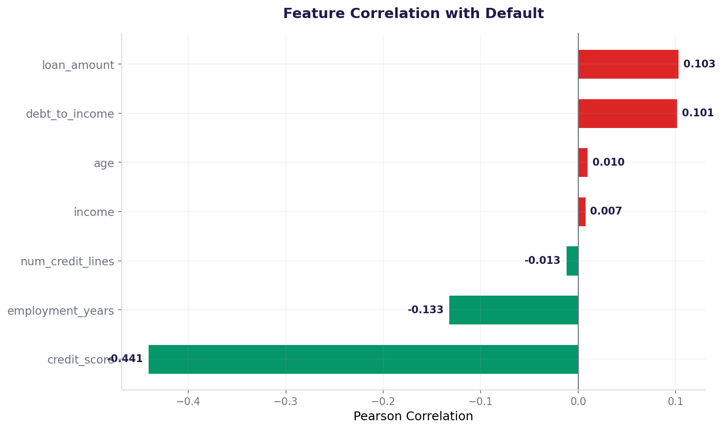
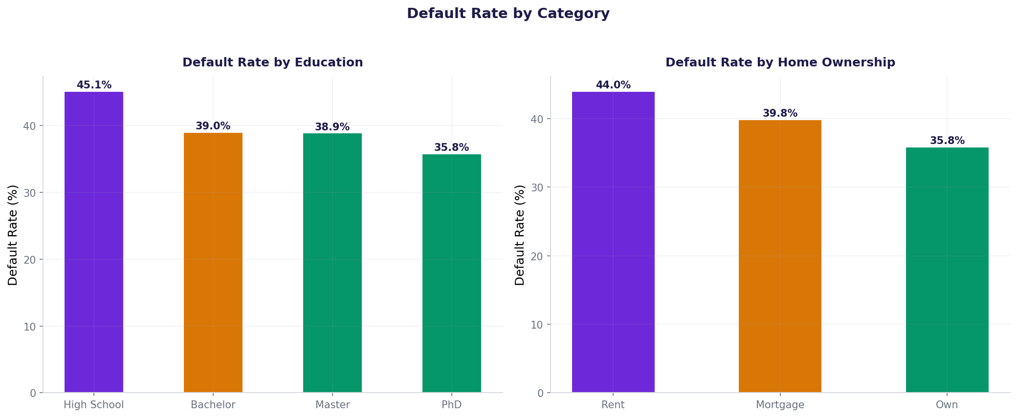
Before modeling, we identify what features matter:
EDA visualizations
Phase 2: Preprocessing and feature engineering
We prepare data for modeling: encode categoricals, scale for distance-based models, split with stratification.
Phase 3: Train all 5 models
Now we train each model on the same train/test split. This ensures fair comparison.
Model 1: Logistic Regression
Model 2: Decision Tree
Model 3: Random Forest
Model 4: XGBoost
Model 5: Support Vector Machine
Phase 4: Model comparison
Side-by-side metrics for all 5 models. Higher is better for all metrics.
| Model | Accuracy | Precision | Recall | F1 Score | AUC |
|---|---|---|---|---|---|
| Logistic Regression | 0.7370 | 0.6868 | 0.6444 | 0.6650 | 0.8029 |
| Decision Tree (d=5) | 0.7120 | 0.6581 | 0.6012 | 0.6284 | 0.7729 |
| Random Forest | 0.7290 | 0.6791 | 0.6272 | 0.6521 | 0.7879 |
| XGBoost | 0.7395 | 0.6934 | 0.6395 | 0.6654 | 0.7988 |
| SVM (RBF) | 0.7360 | 0.6937 | 0.6235 | 0.6567 | 0.7841 |
Phase 5: ROC curve comparison
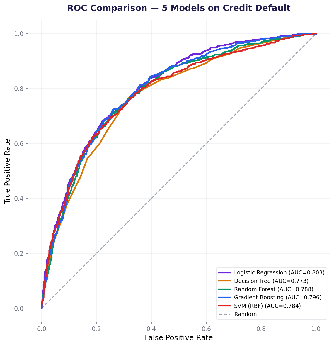
The ROC curve shows true positive rate (recall) vs false positive rate. Higher and to the left = better ranking. AUC is the area under the curve.
Phase 6: Business recommendation for the NeoBank CEO
Now we translate metrics into a business decision. Which model should NeoBank deploy?
The case for Logistic Regression
Recommendation: Deploy Logistic Regression
- Highest AUC (0.8029): Best at ranking applicants by default risk. The bank can set any threshold and trust the ranking.
- Interpretability: Coefficients show exactly which features matter. Credit score has coefficient -1.11, meaning each std-dev increase cuts default log-odds by 1.11. Regulators love this.
- Fast inference: Predicting 10,000 applicants takes milliseconds. XGBoost is slower.
- Stable over time: Linear models are robust to small data shifts. XGBoost can overfit if defaults change.
- Easier maintenance: No hyperparameter tuning needed. No tree pruning. Just retrain on new data.
Why not XGBoost?
XGBoost has higher accuracy (73.95% vs 73.70%) but lower AUC (0.7988 vs 0.8029). Why does this happen? Because the data is mostly linear. Credit score dominates (-0.441 correlation). XGBoost's complexity doesn't help—it's overfitting the noise.
Why not Decision Trees?
Single trees overfit (AUC=0.7729). Although they're interpretable, Random Forest (AUC=0.7879) is a better ensemble. But LR still wins.
What's next: improving the model
After deployment, the real work begins. Here are ways to improve:
- Threshold tuning: The default threshold 0.5 might not be optimal. If false positives (denying good customers) cost more than false negatives, lower the threshold to 0.3. Recompute precision and recall.
- Cost-sensitive learning: Assign weights to classes. FN (approving a defaulter) costs ₹100,000; FP (denying a good customer) costs ₹1,000. Train with these costs.
- Feature engineering: Create interaction features (credit_score × loan_amount). Test polynomial features. Use domain expertise.
- Class rebalancing: 40.5% default rate is imbalanced. Try SMOTE or class weights.
- Retraining schedule: Defaults drift over time (economy, interest rates). Retrain quarterly with new data.
- A/B testing: Deploy LR as the champion. Test XGBoost or RF as challenger models. Measure AUC and business metrics (approval rate, default rate).
How real banks do this
At HDFC, ICICI, SouthBank India: model comparison is quarterly. They maintain champion/challenger frameworks where the production model (champion) is tested against new candidates (challengers). If a challenger has significantly better AUC (usually >1% improvement) and doesn't break regulators' interpretability rules, they promote it. This cycle repeats for years. The production model in 2024 might not be the same as 2020—it evolves with data.
Task: Using Logistic Regression predictions, compute precision and recall at thresholds 0.3, 0.5, and 0.7. At which threshold does recall reach 0.70 (catch 70% of defaulters)? What's the precision at that threshold?
Hint: Use y_pred_proba_lr > threshold to create binary predictions at custom thresholds.
Hint: Recall = TP / (TP + FN). Higher threshold → lower recall, higher precision.
Hint: Loop through thresholds [0.3, 0.5, 0.7] and compute metrics for each.
Interview questions: test your understanding
Quiz: 5 questions to test your knowledge
Cheatsheet: model comparison at a glance
| Model | Best For | Pros | Cons |
|---|---|---|---|
| Logistic Regression | Linear relationships, interpretability | Fast, interpretable, calibrated probabilities, high AUC on linear data | Can't capture non-linearity |
| Decision Tree | Explainability to stakeholders | Visual rules, no scaling needed, handles non-linearity | Overfits easily, high variance |
| Random Forest | Robust predictions, feature importance | Low variance, OOB validation, non-linear | Less interpretable, slower than LR |
| XGBoost | Maximum performance (when data is non-linear) | Handles missing values, regularized, state-of-the-art | Black box, slower, overfits if not tuned |
| SVM | Small datasets, non-linear boundaries | Kernel trick, memory efficient | Slow on large data, no native probabilities, no feature importance |
Common mistakes in model comparison
Key takeaways
Model comparison is about trade-offs, not absolutes.
- Use AUC, not accuracy. AUC measures ranking ability. Accuracy is misleading with imbalanced data.
- Simpler models often win. If logistic regression has high AUC, use it. Don't escalate to forests or boosting without reason.
- Interpretability matters for regulated industries. Banks need to explain credit decisions. XGBoost is a black box.
- Speed matters in production. Logistic Regression predicts 10,000 applicants in milliseconds. XGBoost takes seconds.
- Different models excel at different things. LR: interpretability + calibrated probs. RF: non-linear + feature importance. XGB: max performance. SVM: high-dimensional data.
- Always compare on the same train/test split. Use stratified splitting to preserve class balance.
- Maintain champion/challenger frameworks. Deploy the champion. Test challengers quarterly. Promote if significantly better.
Ready to deploy ML models?
Join the Best AI Program: The AI-Era Analyst — 5 months, fully online, with placement assistance. Week 1 is free.
Explore The AI-Era Analyst →