
In Lesson 20, you used K-Means to segment TelcoMax mall customers into 5 round clusters. But K-Means assumes globular shapes. What if your customers form elongated chains? Hierarchical clustering builds a tree of merges (dendrogram), showing how points group at every level. What if you have outliers—customers who don't fit any normal cluster? DBSCAN finds them and flags them as noise, using density instead of distance.
Same 200 customers, new algorithms, new insights. Let's see how hierarchical and density-based methods reveal hidden patterns.
Agglomerative Clustering: building trees bottom-up
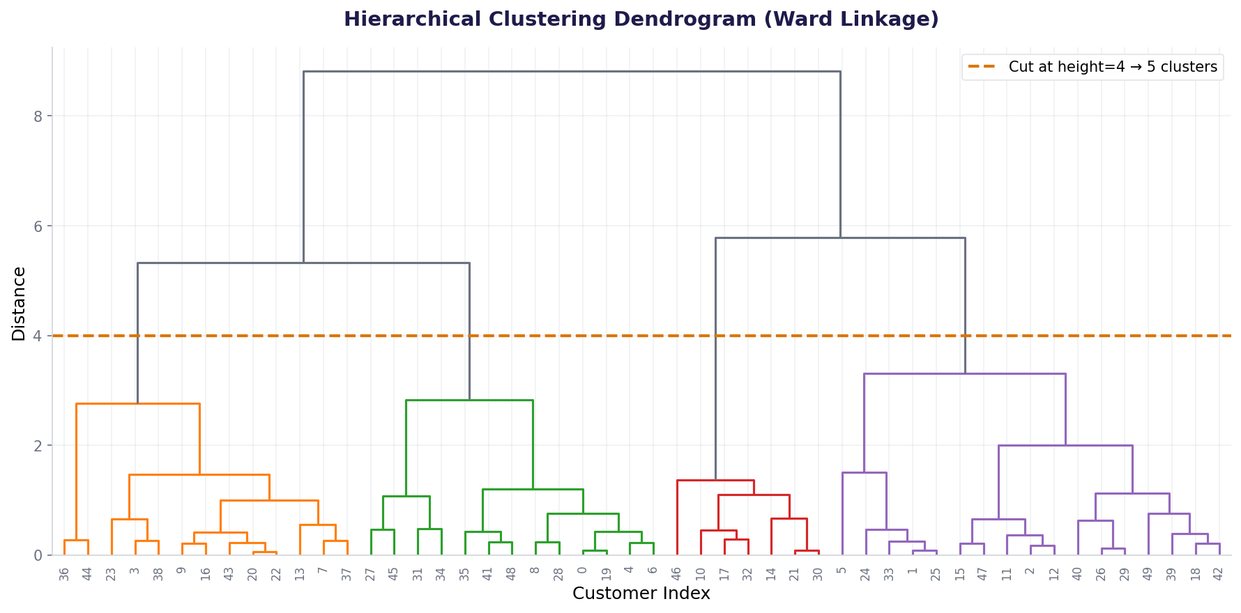
K-Means starts with k centroids and iterates. Agglomerative does the opposite: start with 200 single-point clusters, then merge pairs until you have k clusters. The merging process is tracked in a dendrogram—a tree diagram showing which points/clusters combine and when.
Ward: Minimize within-cluster variance (like K-Means). Most common.
Complete: Distance = farthest pair between clusters (compact clusters).
Average: Distance = mean of all pairwise distances (balanced).
Single: Distance = nearest pair (can create long chains).
Agglomerative Clustering with dendrograms
Let's apply agglomerative clustering to TelcoMax customers using Ward linkage and plot the dendrogram.
Agglomerative finds 5 natural clusters with silhouette 0.4115—similar to K-Means, but the dendrogram reveals the merging hierarchy, which K-Means doesn't.
DBSCAN: density-based clustering for irregular shapes
DBSCAN doesn't assume round clusters. Instead, it groups points by density. A point is a core point if it has at least min_samples neighbors within radius eps. Neighbors of core points form clusters. Points in low-density regions become noise.
Core point: At least min_samples points (including itself) within eps radius.
Border point: Not core, but within eps of a core point (assigned to its cluster).
Noise point: Neither core nor border (outlier, cluster label = -1).
| Parameter | Meaning | How to choose |
|---|---|---|
eps |
Radius of neighborhood search | Too small: everything is noise. Too large: one big cluster. Plot k-distance graph; pick knee. |
min_samples |
Points needed (including self) to be core | Usually = dimensions + 1. For 2D: min_samples=3 or 5. |
DBSCAN with eps sweep
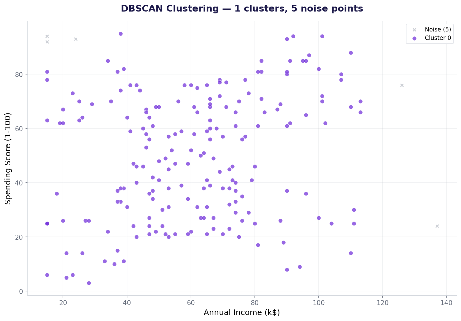
DBSCAN is sensitive to eps. Let's sweep different eps values and observe cluster counts and noise points.
At eps=0.3: tight clustering, many outliers (47 noise points). At eps=0.5+: everything merges into one giant cluster. The sweet spot depends on your domain and what "outlier" means.
DBSCAN eps sweep: visualizing the trade-off
Hierarchical vs. DBSCAN vs. K-Means
| Aspect | K-Means | Hierarchical (Agglomerative) | DBSCAN |
|---|---|---|---|
| Cluster shape | Round (convex) | Any shape (via dendrogram) | Any shape (density-based) |
| Number of clusters | Fixed (k given) | Choose by cutting dendrogram | Emergent (from eps, min_samples) |
| Outliers | Forced into clusters | Assigned to nearest cluster | Labeled as noise (-1) |
| Dendrogram | No | Yes (full merge history) | No |
| Scalability | Fast (O(nk) per iter) | Slow (O(n²) or O(n² log n)) | Slow (O(n²) without spatial index) |
Also used in...
Domain Spotlight
How AI systems use this
Large language models don't cluster text directly, but clustering powers retrieval and recommendation. DBSCAN finds clusters of similar documents; hierarchical clustering helps organize knowledge hierarchically (like a taxonomy). Outlier detection via DBSCAN catches malformed inputs before they reach the model.
Task: Load mall_customers.csv. Scale it. Apply DBSCAN with eps=0.4, min_samples=5. Count clusters (exclude noise). Print noise count. Compare: which eps (0.3, 0.4, 0.5) gives the best balance of cluster compactness and outlier detection?
Hint 1: Use DBSCAN(eps=0.4, min_samples=5).fit_predict(X_scaled)
Hint 2: Count noise: list(labels).count(-1)
Hint 3: Clusters: len(set(labels)) - (1 if -1 in labels else 0)
Hint 4: For 2D data, silhouette ignores noise: filter labels before computing.
Interview questions: test your understanding
Quiz: 5 questions to test your knowledge
Cheatsheet: hierarchical & density clustering at a glance
| Algorithm | Code | Best for |
|---|---|---|
| Agglomerative (Ward) | AgglomerativeClustering(n_clusters=k, linkage='ward') |
Exploring cluster hierarchies, moderate data |
| Dendrogram | dendrogram(linkage(X, 'ward')) |
Visualizing merges, choosing k |
| DBSCAN | DBSCAN(eps=0.5, min_samples=5).fit_predict(X) |
Irregular clusters, outlier detection |
| Linkage types | linkage='ward'|'complete'|'average'|'single' |
Ward=variance, complete=compact, average=balanced, single=chains |
| Choose eps (DBSCAN) | Plot k-distance graph, find elbow | No universal rule; domain and data shape matter |
Common mistakes: what breaks and how to fix it
Key takeaways
Clustering is not one-size-fits-all. Choose wisely based on your data and goals.
- Hierarchical clustering: Build a tree of merges. Dendrograms let you explore cluster hierarchies without pre-specifying k.
- Linkage types matter: Ward (variance), complete (compact), average (balanced), single (chains). Ward is most common.
- DBSCAN finds irregular shapes: No assumption of round clusters. Naturally handles outliers (noise points).
- eps is critical for DBSCAN: Too small = everything is noise. Too large = one giant cluster. Use k-distance graph or sweep.
- Scale before density-based methods: DBSCAN depends on distance; unscaled features bias results.
- K-Means vs. Hierarchical vs. DBSCAN: Use K-Means for speed and round clusters. Hierarchical for exploration. DBSCAN for irregular shapes and outliers.
Ready to master unsupervised learning?
Join the Best AI Program: The AI-Era Analyst — 5 months, fully online, with placement assistance. Week 1 is free.
Explore The AI-Era Analyst →