
Aisha is a product manager at M-Kopa Solar in Nairobi, an energy access startup serving underbanked customers across Kenya. She has 1,338 customer records with 7 features: age, BMI, smoker status, region, children, sex, and monthly charges. The product team asks: "Should we deploy a neural network to predict next month's charges, or stick with Random Forest?" Aisha decides to build both and compare. The answer surprises her: on small tabular data, the simpler model wins. This lesson teaches you why.
By the end, you'll understand the fundamental trade-off: deep learning needs scale to shine, but traditional ML dominates on small, structured datasets. You'll also learn when each approach wins—images vs tables, thousands vs billions of samples.
📊 Meet the data: Insurance charges
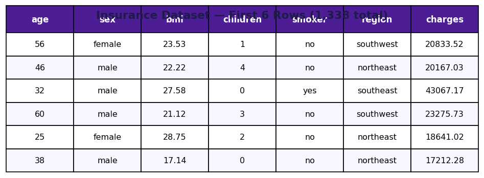
We'll use the Insurance dataset — 1,338 real customer records with 7 features. The goal: predict medical charges from age, BMI, smoking status, and more. This is the same dataset used across Arc A and B.
The fundamental difference
Traditional Machine Learning
Optimized for: Structured, tabular data (spreadsheets, CSVs, databases)
Feature engineering: You manually design features. For example: "Is this customer a smoker? Create a binary smoker column."
Algorithms: Decision trees, Random Forest, XGBoost, SVM, linear models
Training time: Seconds to minutes
Interpretability: Easy. Feature importance shows which columns matter most.
Deep Learning
Optimized for: High-dimensional, unstructured data (images, text, audio, video)
Feature learning: The model automatically learns features. A CNN learns edges → shapes → objects without you telling it what to look for.
Algorithms: Neural networks, CNNs, RNNs, Transformers (like GPT)
Training time: Hours to days (needs GPUs)
Interpretability: Hard. The model is a "black box"—you can't easily say why it made a decision.
The data regime quadrants: where each approach wins
Small data + Tabular: Traditional ML wins. You have 1k–100k rows and 10–100 columns. Random Forest or XGBoost fits in seconds without overfitting.
Small data + Images: Transfer learning wins. You have 1k–10k images. Use a pretrained CNN (trained on ImageNet with millions of images), then fine-tune it on your data.
Large data + Tabular: Deep learning can compete, but carefully. You need 1M+ rows and careful regularization. Gradient boosting (XGBoost, LightGBM) often still wins.
Large data + Images/Text: Deep learning dominates. You have 100k–billions of samples. CNNs and Transformers learn hierarchical representations that traditional ML can't match.
Case study: Random Forest on M-Kopa Solar charges
Aisha starts simple: train a Random Forest on the customer data. No neural network, no GPUs—just 100 decision trees voting.
Case study: PyTorch neural network on the same data
Now Aisha tries a neural network: a multi-layer perceptron with batch normalization. Same 1,338 training samples, but this time the model has 2,561 parameters to learn.
Performance comparison: Random Forest vs PyTorch
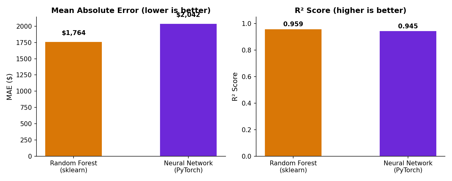
Both models achieve >94% R², but Random Forest is cleaner on this small dataset. The neural network overfits: it learns training patterns that don't transfer to test data.
Training loss curves: why the neural network struggles
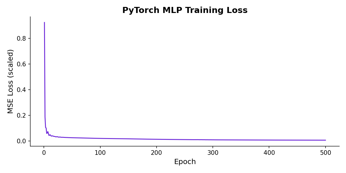
Watch the learning trajectories. Random Forest's training is stable—it makes one-shot decisions for each split. The neural network's loss bounces around, showing the optimizer fighting with 2,561 parameters and only 1,070 training samples.
Actual vs predicted: scatter plot reveals overfitting
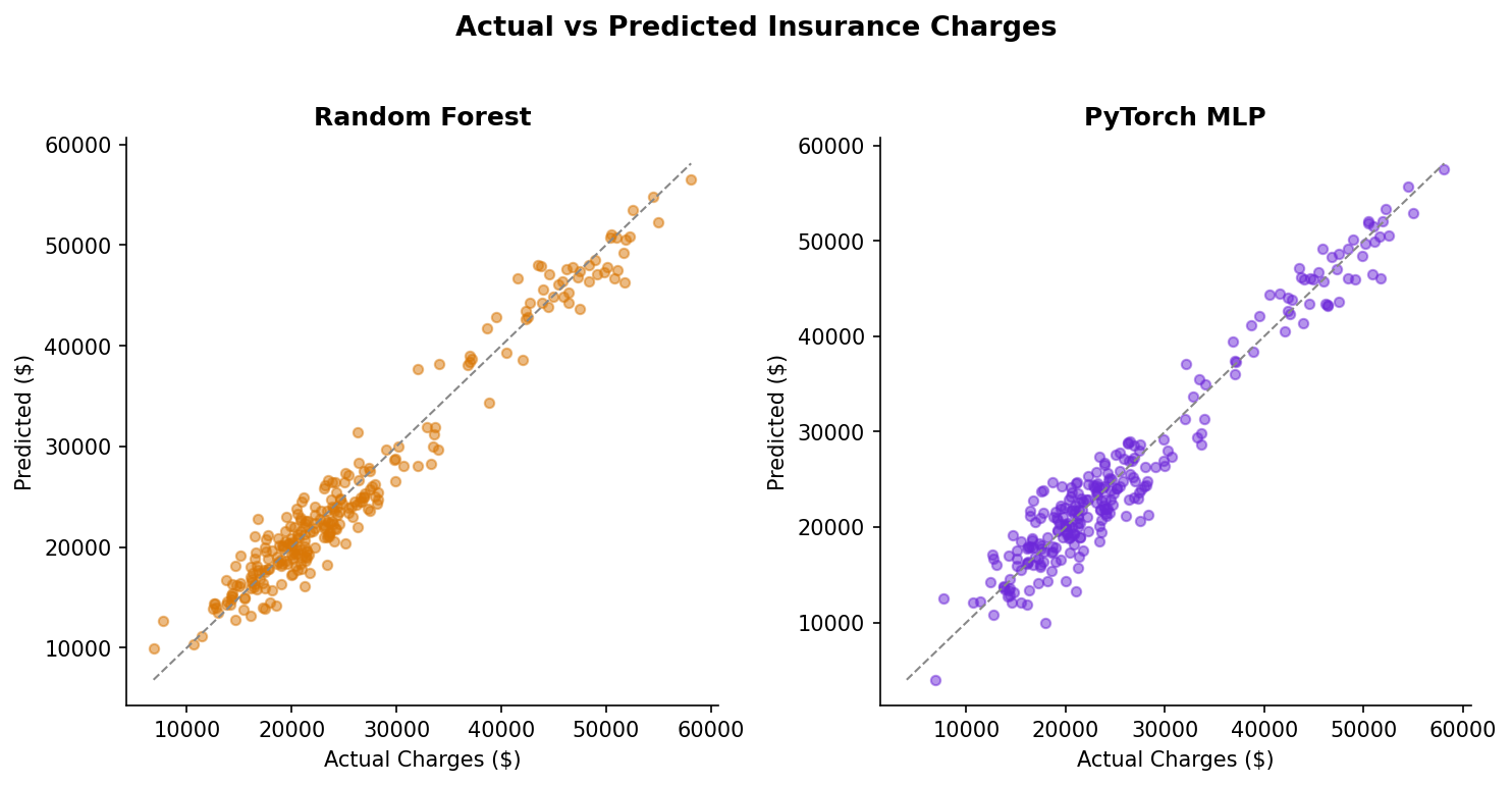
Points close to the dashed diagonal line = good predictions. Random Forest's points cluster tighter; PyTorch's scatter more. This visual confirms the 278 MAE gap.
When does Random Forest win vs deep learning?
A framework for choosing. On small tabular datasets, traditional ML algorithms have built-in inductive biases that match the problem structure. Neural networks need scale to justify their complexity.
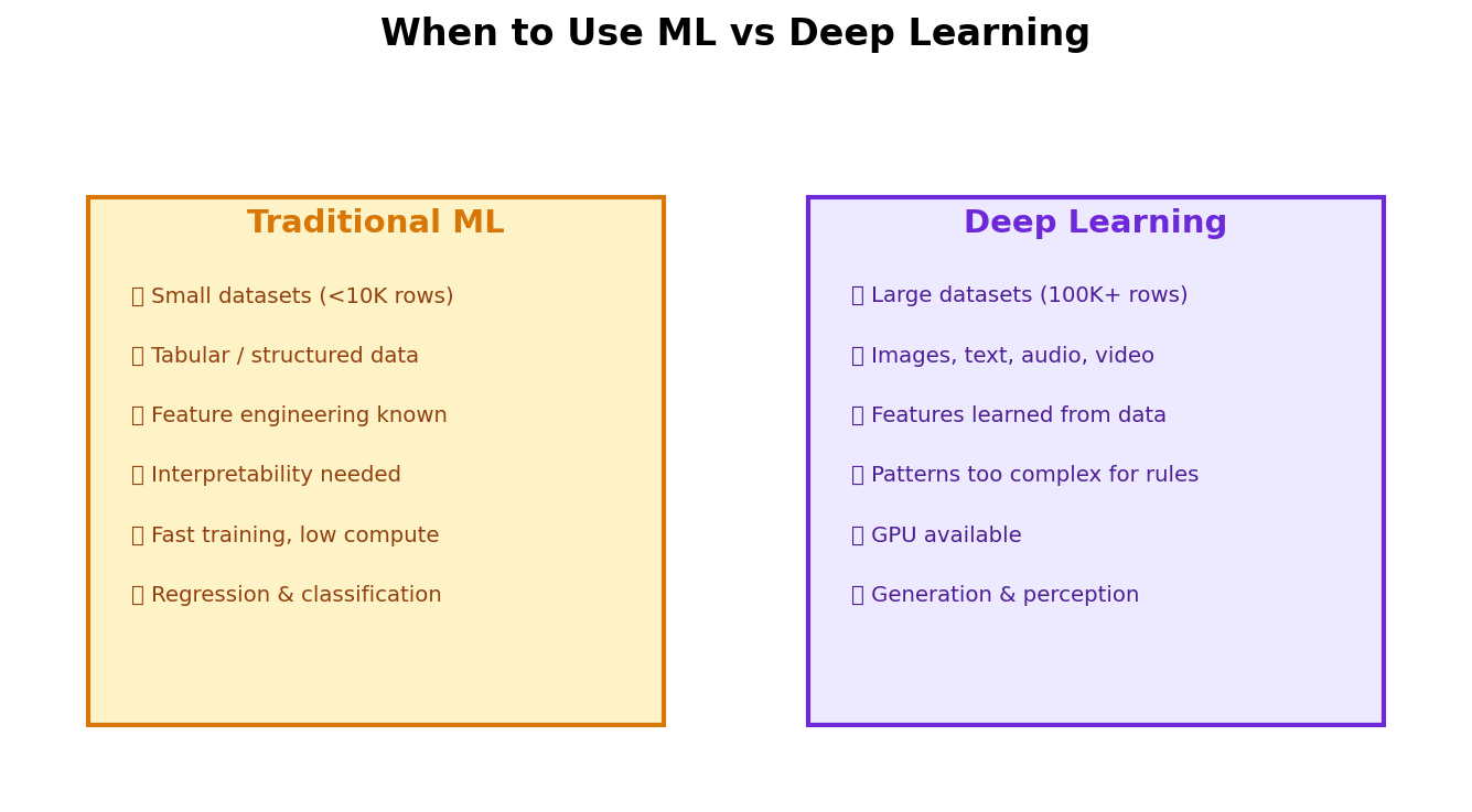
Why Random Forest wins on small tabular data
1. Parameter efficiency
Random Forest with 100 trees has ~100 "rules" (splits). A neural network with 2,561 parameters is trying to memorize individual patterns. On 1,338 samples, RF's bias toward simple splits matches the data.
2. Built-in regularization
RF's ensemble voting is a form of regularization: one tree overfits, but 100 trees voting cancel out noise. Dropout in neural networks tries to achieve similar ensemble behavior but less naturally.
3. Feature interactions are already handled
RF learns splits like "if smoker AND age > 40, predict high charges." You don't manually code this. Neural networks can learn it, but need more data to do so robustly.
4. Non-linear boundaries without overfitting
Decision trees partition space into rectangles. On 7 features (age, BMI, smoker, region, children, sex, charges), this is natural. A neural network needs many layers and careful tuning to avoid overfitting to noise.
5. Training speed
RF fits in seconds. You can experiment with different hyperparameters quickly. Neural networks take minutes per training run, slowing iteration.
When deep learning wins: the reasons
1. Image data (high-dimensional spatial)
A 224×224 pixel image = 50,176 raw features. Random Forest can't build useful trees—the feature space is too large and pixels are meaningless in isolation. A CNN learns that neighboring pixels form edges, edges form shapes, shapes form objects. This hierarchical learning is DL's superpower.
2. Text data (sequential, context matters)
Word order matters: "not good" vs "good" have opposite meanings. Random Forest treats text as bag-of-words (losing order). Transformers (like ChatGPT) use attention to capture context: "what words should I pay attention to right now?" On millions of documents, this learned attention beats hand-crafted features.
3. Audio data (temporal patterns)
A waveform is a sequence of 16,000 samples per second. Traditional ML uses hand-engineered features (MFCCs). LSTMs and RNNs learn temporal dependencies directly: "after this pattern, that sound usually follows." On large speech datasets, this beats hand-crafted features.
4. Large datasets (where DL's scaling laws kick in)
Empirical scaling law: test loss ∝ N^(-0.07). With 1B examples, deep learning accuracy scales smoothly while traditional ML plateaus. GPT, DALL-E, etc. prove this at billion-example scale.
5. Feature learning at scale
With 100k+ images, a CNN learns useful features (edges, textures, shapes) that transfer to new tasks. You can't hand-engineer 10,000 features that general purpose. But a neural network trains on billions of unlabeled examples and learns them automatically.
Deep learning downsides: not a silver bullet
1. Needs scale: You need 100k+ samples for most DL tasks. Aisha has 1,338. She can't justify the overhead.
2. Slow to train: RF fits in seconds. PyTorch took minutes. At scale (billions of parameters, billions of samples), training takes weeks and costs thousands in GPU time.
3. GPU dependency: Training a CNN or Transformer on CPU is agonizing. RF runs fine on CPU. This adds infrastructure cost.
4. Hyperparameter hell: RF has ~5 hyperparameters (tree depth, n_trees, min_samples_leaf). Neural networks have 20+ (learning rate, batch size, layer sizes, dropout, weight decay, optimizer, activation functions, ...). Wrong choices tank performance.
5. Black box: Which features matter in your RF? Easy—check feature_importances_. Which neurons learned what? Hard. Adversarial examples exist: tiny pixel changes that fool networks but don't fool humans.
6. Requires careful regularization: Dropout, batch norm, early stopping, weight decay. Get any wrong and the model overfits. RF is naturally robust.
Decision framework: choosing the right approach
Ask these questions in order:
| Question | Answer → Choose Traditional ML | Answer → Choose Deep Learning |
|---|---|---|
| Data type? | Tabular (spreadsheet, CSV) | Images, text, audio, video |
| How many samples? | <100k | 100k+ |
| Feature engineering? | Easy (domain knowledge works) | Hard (patterns hidden in raw data) |
| Interpretability critical? | Yes (healthcare, finance, law) | No (recommendation, image labeling) |
| Compute budget? | Limited (CPU, hours) | High (GPUs, days) |
| Time to deploy? | Days (tune hyperparameters, deploy) | Weeks (experiment, tune, debug) |
Rule of thumb: Start with traditional ML (RF, XGBoost). If performance hits a ceiling and you have more data, try deep learning. Premature optimization is the root of engineering overhead.
How AI systems use this
ChatGPT uses deep learning (Transformers) because language is high-dimensional and context-dependent. A Random Forest treating each word independently would destroy meaning: "not bad" vs "bad" would look identical. Transformers learn attention: "which tokens should I focus on?" This learned attention is what makes LLMs work. But for your M-Kopa Solar charges prediction, RF's simple split rules are all you need. AI complexity should match the problem.
Also used in...
Domain Spotlight
Task: You have 50k customer records with 50 tabular features AND 5 product images per customer. Design a model architecture that combines both. Hint: don't use just one approach.
Hint 1: Use a CNN on images (learns visual features automatically)
Hint 2: Use a feedforward NN or RF on tabular features
Hint 3: Concatenate learned representations before final prediction layer
Expected architecture: [Images] → CNN → flatten → [Dense layer] concatenate [Tabular features] → Dense layer → [Output]
Why this works: Let each modality use its optimal algorithm. CNN learns visual patterns; tabular encoder captures demographic/transactional logic. Together they're stronger than either alone.
Interview questions: test your understanding
Quiz: 5 questions to test your knowledge
Cheatsheet: Traditional ML vs Deep Learning at a glance
| Aspect | Traditional ML | Deep Learning |
|---|---|---|
| Best for | Tabular (CSV, spreadsheets) | Images, text, audio, video |
| Data needed | 100–100k samples | 100k–billions samples |
| Training time | Seconds to minutes (CPU) | Hours to days (GPU) |
| Requires GPU? | No | Usually yes |
| Interpretable? | Yes (feature importance) | No (black box) |
| Hyperparameters | Few (tree depth, n_trees) | Many (lr, batch size, layers) |
| Example algorithms | Random Forest, XGBoost, SVM | CNN, RNN, Transformer |
| Feature engineering | Manual, domain-knowledge based | Automatic (learned representations) |
Common mistakes: avoid these traps
Key takeaways
Aisha learned a painful but valuable lesson at M-Kopa Solar: the fancier algorithm doesn't always win.
- Size matters: With 1,338 samples, Random Forest is optimal. Neural networks shine at 100k+ samples.
- Data type matters: Tabular data → Traditional ML. Images/text → Deep Learning.
- Interpretability matters: Healthcare and finance need transparent models. RF's feature importance beats NN's black box.
- Train time matters: RF fits in seconds, allowing rapid iteration. NN takes minutes, slowing experimentation.
- Measure on test data, always: Train metrics lie. Only test metrics reveal generalization.
- Start simple, add complexity only when needed: RF first. If it hits a ceiling and you have more data, then try deep learning.
- Hybrid approaches work: CNN on images + RF on tabular = better than either alone.
You've compared Random Forest to neural networks.
Now master both in production.
Join the Best AI Program: The AI-Era Agentic Engineer — 5 months, fully online, with placement assistance. Week 1 is free.
Explore The AI-Era Agentic Engineer →