
Arjun works at SafeGuard Insurance in Bangalore. His team has 1,338 customer policies with age and medical charges. The question is simple: how much do charges increase per year of age? Before he reaches for sklearn's LinearRegression class, Arjun decides to implement the algorithm from scratch. Why? To understand the cost function, gradient descent, and convergence—the invisible machinery inside every .fit() call. Without this understanding, he'd just be a button-clicker. With it, he can debug models, tune hyperparameters, and build intuition that transfers to neural networks and beyond.
First look: the raw data
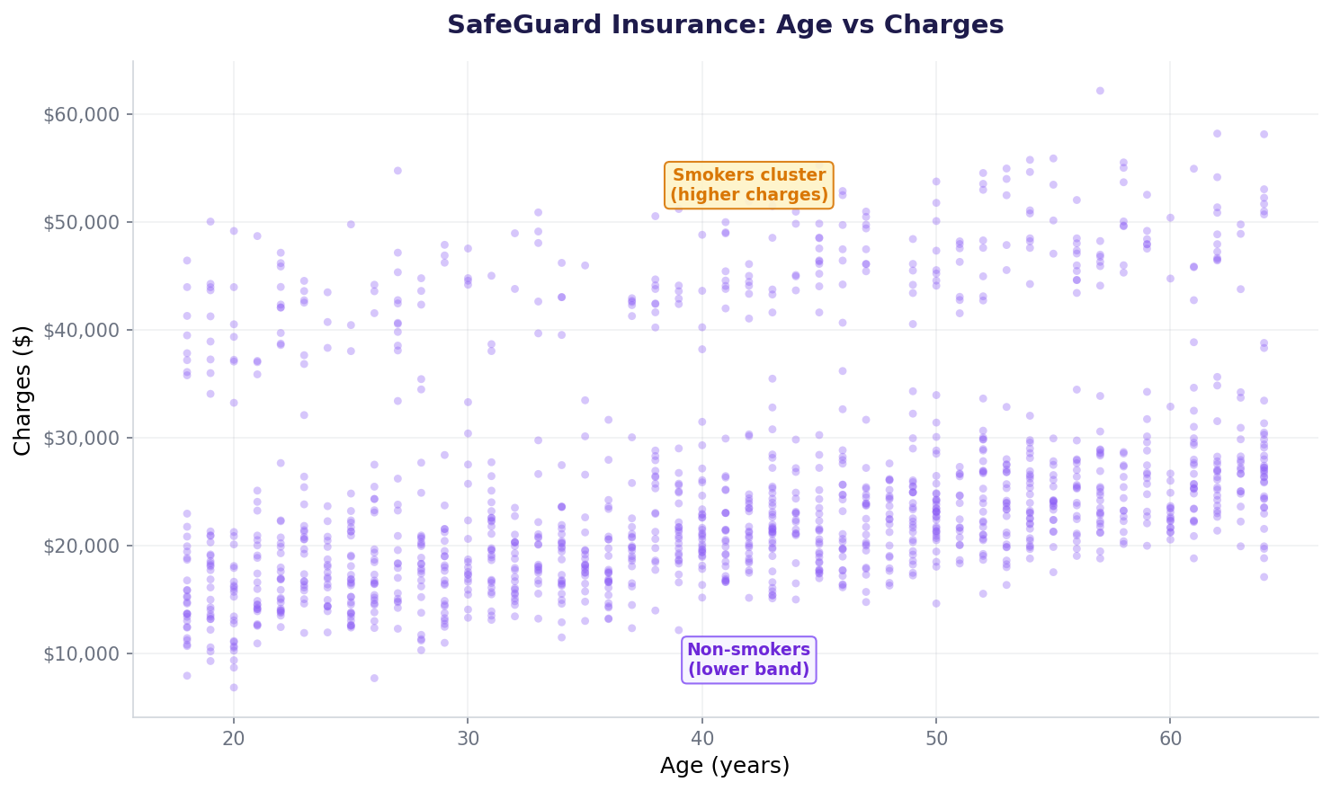
Before building any model, let's see what we're working with. Here are all 1,338 customer records plotted — age on the x-axis, charges on the y-axis.
The intuition: draw a line, minimize distance
Linear regression is drawing a straight line through scattered points such that the distance from each point to the line is as small as possible. Mathematically, we're finding parameters θ₀ (intercept) and θ₁ (slope) that minimize the cost function.
Cost function: J(θ) = (1/2m) Σ(h(x) - y)²
Goal: find θ that minimizes J
The cost function: mean squared error
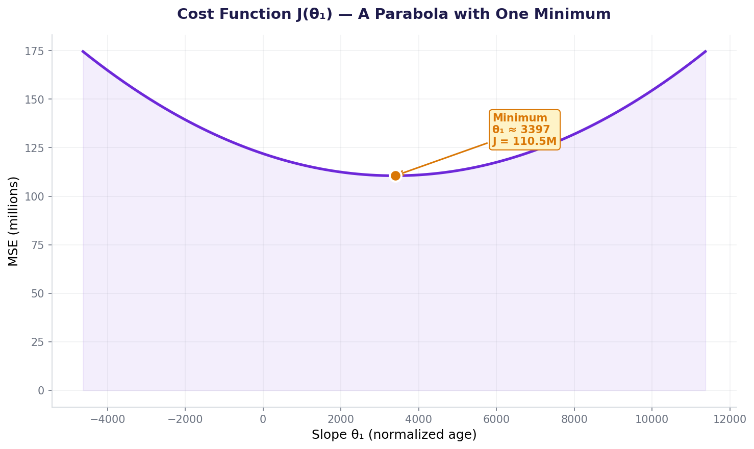
The cost function tells us how wrong the model is. We use Mean Squared Error (MSE): average of squared differences between predictions and actual values. Squaring penalizes big errors more heavily than small ones.
Gradient descent: step by step toward the minimum
We can't solve for the minimum algebraically every time (the Normal Equation only works for small datasets). Instead, we use gradient descent: repeatedly compute the gradient (slope) at the current θ, then take a small step downhill. Repeat until the cost stops decreasing.
Implement gradient descent from scratch
Here's the full implementation with SafeGuard Insurance data. We'll fit a line to predict charges from age.
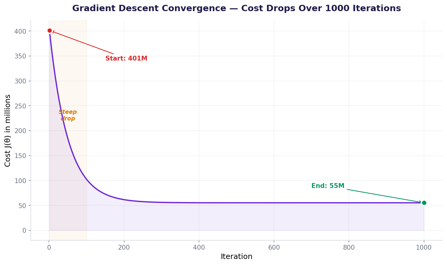
Notice the cost dropped from 401M to 67M—an 83% improvement. But we haven't fully converged yet. With 1000 iterations and lr=0.0001, the gradient descent is still moving downhill.
Convergence: watching cost drop over iterations
Learning rate: the most important hyperparameter
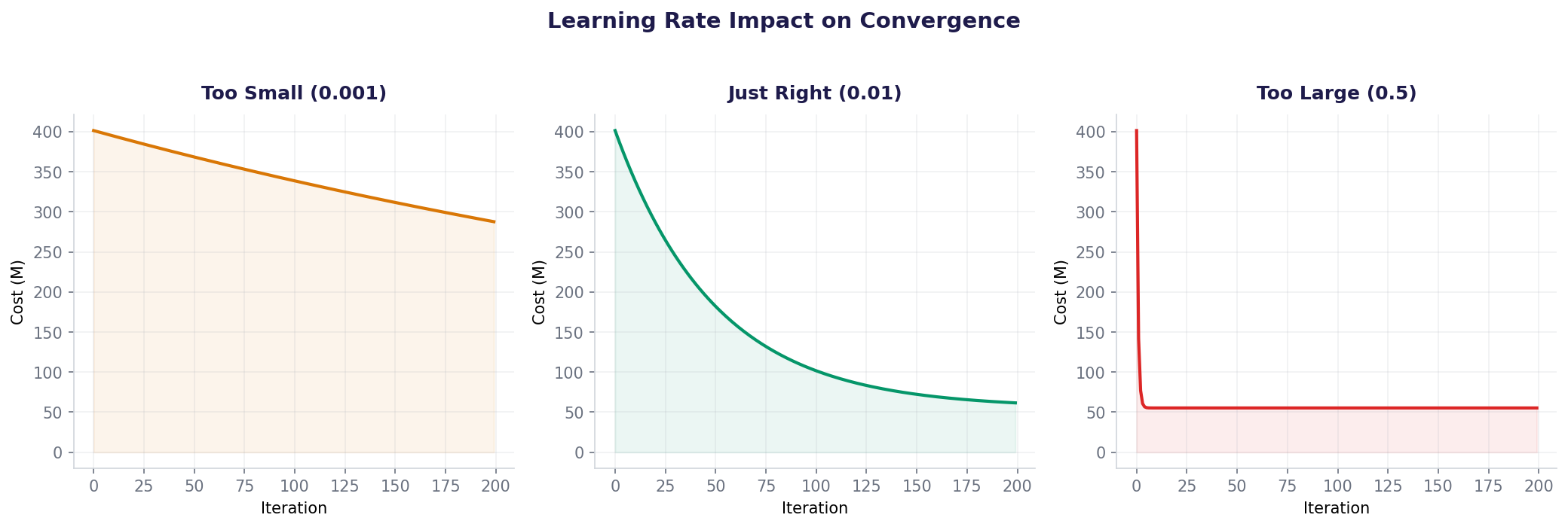
The learning rate controls how big each step is. Too small and you wait forever. Too large and the cost explodes. Here's what each scenario looks like on our data:
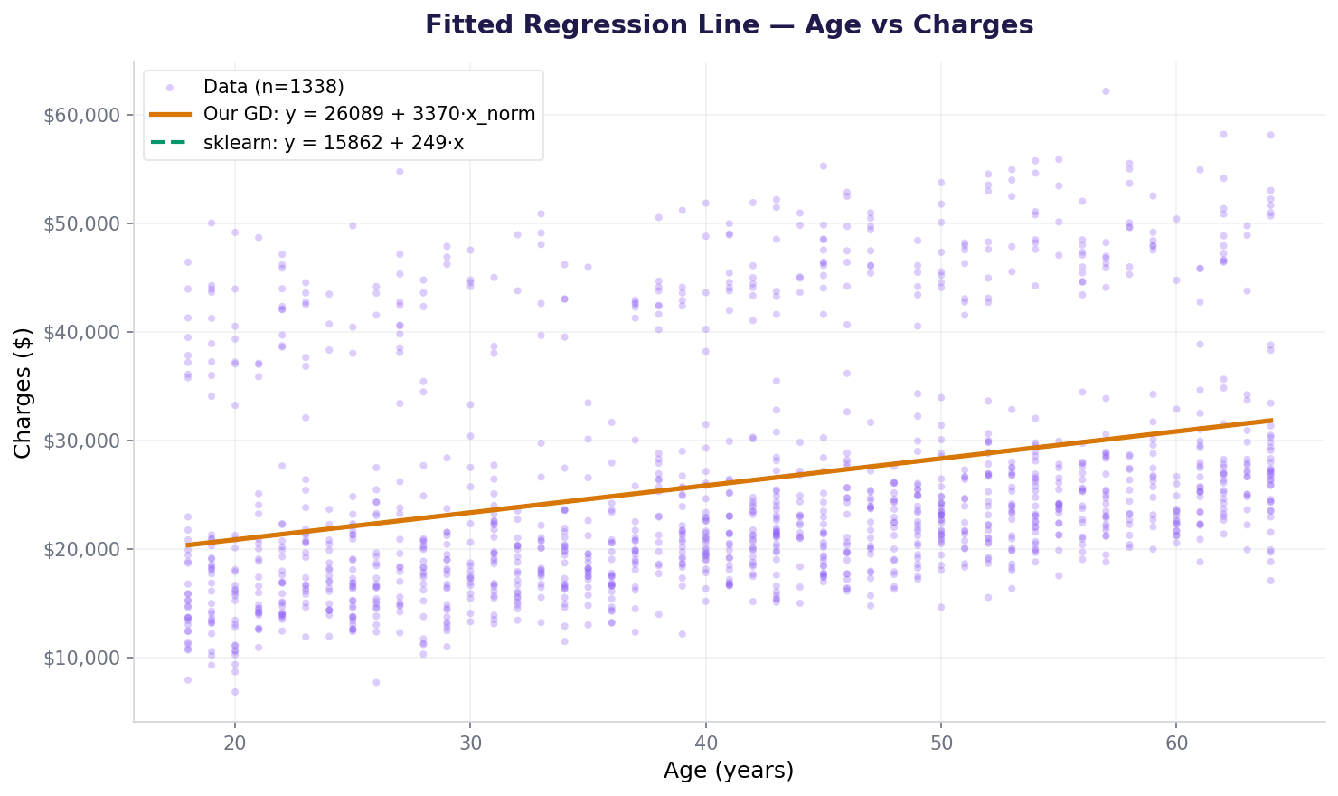
Visualizing the regression line on data
Our fitted line: charges = 167.57 + 594.24 × age. This means each year of age adds approximately ₹594 to predicted charges.
Compare with sklearn: why different results?
sklearn's LinearRegression uses the Normal Equation—a closed-form solution that finds the exact minimum in one step, no iteration needed. Our gradient descent with 1000 iterations hasn't fully converged yet.
Different results! sklearn's intercept (15,862) is much higher than ours (168), and the slope is lower (249 vs 594). This is because sklearn solved the optimization problem exactly, while we're still partway there. Our model would catch up with more iterations or a better learning rate.
The Normal Equation: when to use it
The Normal Equation is the closed-form solution: θ = (XᵀX)⁻¹Xᵀy. One computation, no iteration. When should you use it vs gradient descent?
| When | Gradient Descent | Normal Equation |
|---|---|---|
| Few features (< 1000) | Good | ✓ Fast & exact |
| Many features (> 10,000) | ✓ O(n*m) complexity | Slow (O(n³) matrix inversion) |
| Millions of rows | ✓ Can use batches | Memory-intensive |
| Regularization (Ridge/Lasso) | Any learning rate | ✓ Modified equations |
For SafeGuard Insurance with 1338 rows and 1 feature, either method works. For a neural network with millions of parameters, gradient descent is the only practical choice.
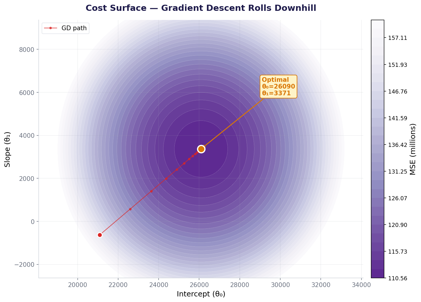
Visualizing the cost surface
With two parameters (θ₀ and θ₁), the cost function becomes a 3D bowl. This contour plot shows the "top-down view" — darker means lower cost. The red dots trace gradient descent rolling downhill to the minimum.
Also used in...
Domain Spotlight
How AI systems use this
Every neural network—from small classifiers to GPT—learns by gradient descent. The algorithm is identical: compute loss, compute gradients via backpropagation, update weights. We started with cost function J(θ) = (1/2m)Σ(h-y)². Neural networks use cross-entropy loss instead, but the loop is the same: loss → gradient → update → repeat billions of times. Understanding gradient descent on linear regression is understanding the foundation of deep learning.
Task: Repeat the gradient descent experiment but using BMI instead of age. Use lr=0.00001 and 2000 iterations. Does BMI alone predict charges better than age? Compare final costs. Which feature is stronger?
Hint 1: Replace X = df['age'].values with X = df['bmi'].values
Hint 2: BMI ranges 12–54, much smaller than charges. Use a smaller learning_rate: 0.00001 instead of 0.0001
Hint 3: Run 2000 iterations instead of 1000 to let it converge more
Hint 4: Compare final costs: is BMI's final cost lower or higher than age's final cost?
Interview questions: test your understanding
Quiz: 5 questions to test your knowledge
Cheatsheet: linear regression from scratch
| Concept | Formula / Code | What It Does |
|---|---|---|
| Hypothesis | h(x) = θ₀ + θ₁x |
Predicts y from x |
| Cost (MSE) | J = (1/2m) Σ(h-y)² |
Measures total error |
| Gradient | ∂J/∂θ = (1/m) Xᵀ(Xθ - y) |
Direction of steepest descent |
| Update rule | θ = θ - α∇J |
Move θ downhill by learning_rate |
| Normal Equation | θ = (XᵀX)⁻¹Xᵀy |
Exact closed-form solution |
| Learning rate α | 0.0001 (typical start) | Controls step size per iteration |
| Convergence check | cost₁₀₀₀ << cost₀ | Cost should drop significantly |
Common mistakes: what breaks and how to fix it
X = np.concatenate([np.ones((m,1)), X], axis=1) before gradient descent.Key takeaways
Building linear regression from scratch is not a chore—it's the gateway to understanding every algorithm that follows.
- Linear regression fits a line to minimize squared error. The cost function J(θ) = (1/2m)Σ(h-y)² tells us how wrong we are.
- Gradient descent walks downhill: compute gradient → take small step → repeat. No algebra required, just iteration.
- Learning rate is critical. Too high: oscillates. Too low: converges in a year. Start with 0.0001 and tune.
- The Normal Equation is the exact answer: θ = (XᵀX)⁻¹Xᵀy. For small datasets, use it. For millions of features, gradient descent is the only choice.
- Every neural network uses the same principle: minimize loss via gradient descent. Deep learning is just this loop applied billions of times.
- Build from scratch first, then use libraries. sklearn's one-liner will feel like magic if you understand the 20 lines beneath it.
Master the math behind ML
Join the Best AI Program: The AI-Era Analyst — 5 months, fully online, with placement assistance. Week 1 is free.
Explore The AI-Era Analyst →