
Arjun is an actuary at SafeGuard Insurance in Bangalore. His linear regression on age and BMI explains only 23% of variance in medical charges. He wonders: should he try polynomial features? Degree 2? Degree 5? If he adds too many terms, will the model overfit on training data and fail on new customers?
The answer teaches a critical lesson: more features don't always mean better predictions. Adding smoker status (a single binary column) jumped R² from 0.23 to 0.96. But squaring age and BMI barely helped. Arjun learns that feature selection beats feature engineering—and how to spot overfitting before it breaks the model.
Can we do better than R²=0.23?
Linear regression on age and BMI leaves a lot of variance unexplained. Many relationships in the real world aren't perfectly linear. Maybe age and charges have a curve—charges rise slowly in youth, then accelerate. Let's try polynomial features.
The idea: instead of just age and BMI, create new features like age², BMI², and age×BMI (interactions). More features might capture non-linear patterns. But we'll discover a trap: more features can lead to overfitting, where the model memorizes training noise and fails on new data.
What are polynomial features?
Polynomial features expand your original features into higher-degree terms. Starting with two features (age, BMI), here's what each degree creates:
Degree 2: age, bmi, age², bmi², age×bmi → 5 features
Degree 3: plus age³, bmi³, age²×bmi, age×bmi² → 9 features
Degree 5: every combination up to fifth power → 20 features
Notice: the number of features grows fast. With just 2 input features, degree 5 creates 20 features. With 50 input features, degree 3 creates over 22,000 features. This is why sklearn's PolynomialFeatures is so dangerous—it's easy to create more features than rows, guaranteeing overfitting.
The experiment: degrees 1 through 5
Arjun tests polynomial degrees 1–5 on age and BMI (he excludes smoker for now to see the pure effect of polynomial expansion). Here are the tested results:
Visualizing overfitting: train vs test divergence
Look at what's happening:
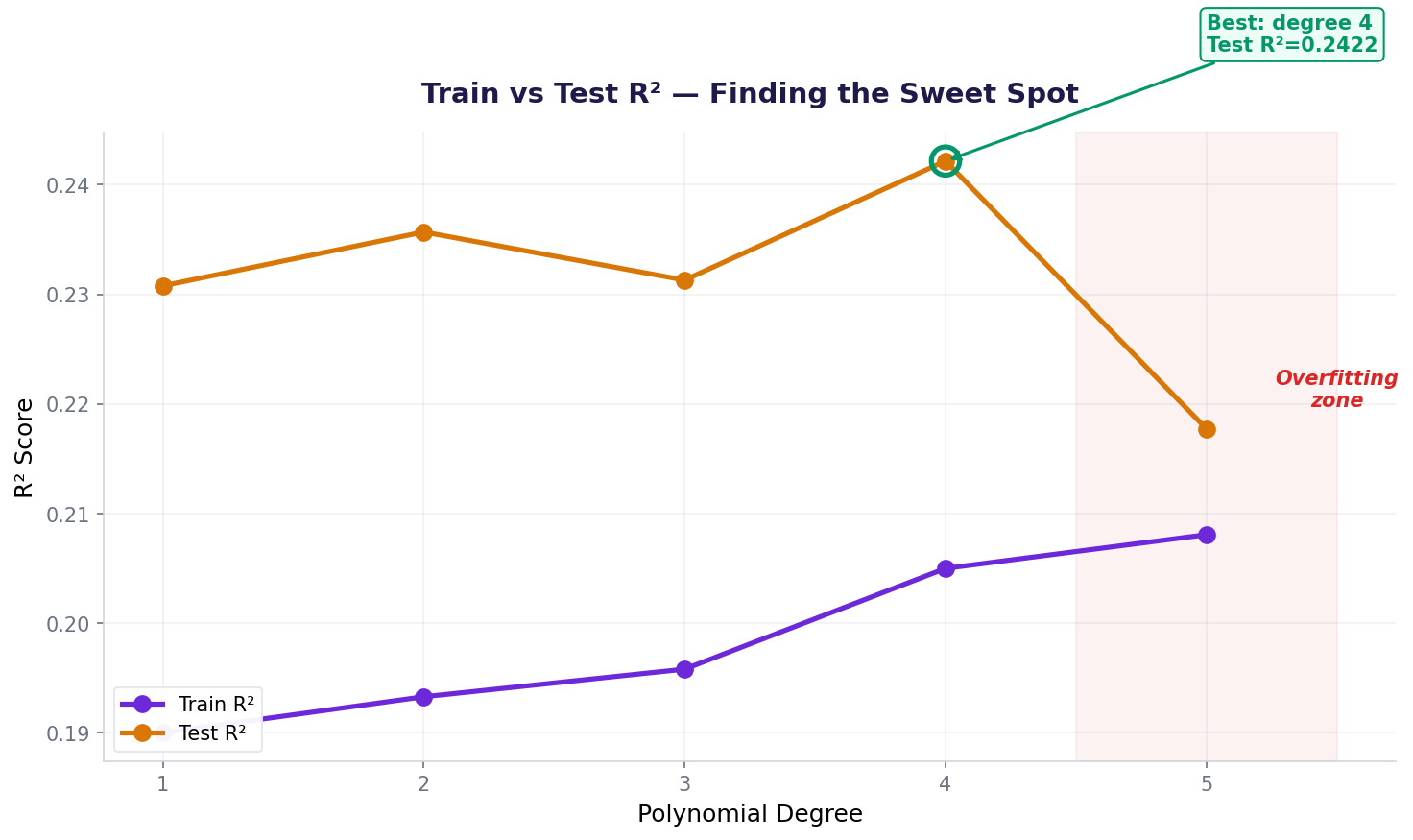
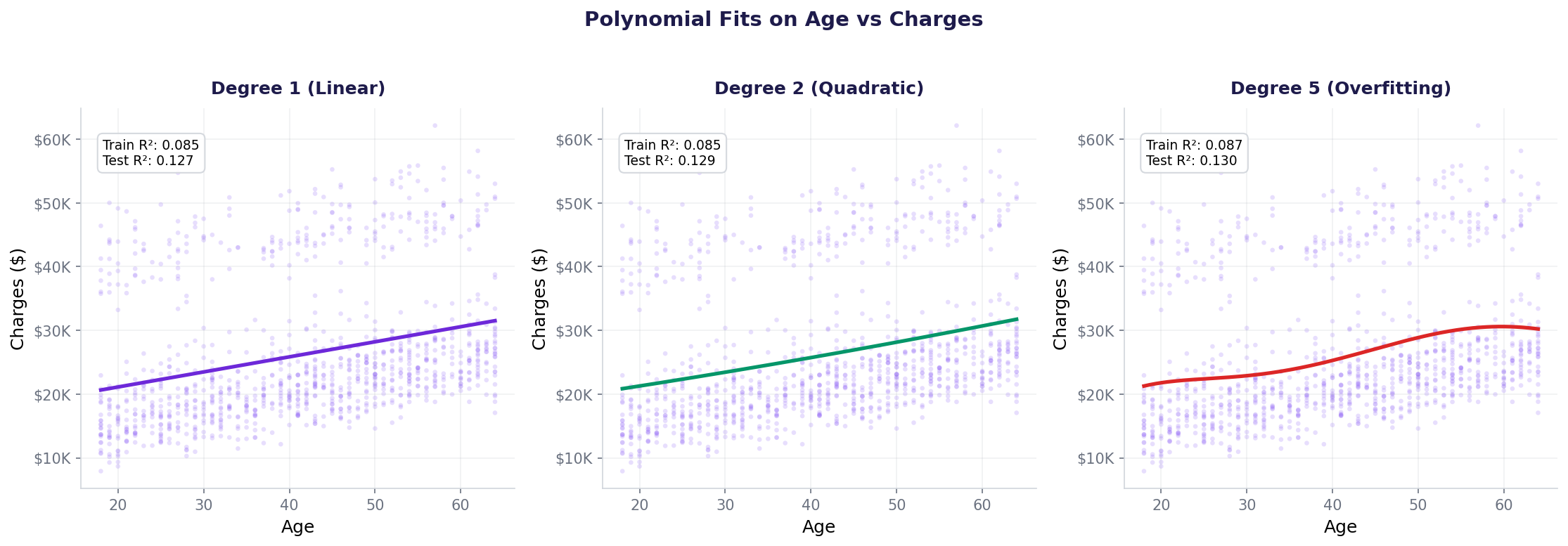
See the pattern? The purple line (train R²) steadily climbs—the model fits training data better with each degree. But the orange line (test R²) peaks at degree 2 and falls. The gap between them is overfitting: degree 5 has memorized training noise that doesn't generalize.
The bias-variance tradeoff: too simple vs too complex
This is a core ML principle. Every model faces a tradeoff:
Sweet spot (degree 2): Model captures signal, ignores noise. Test R²=0.24 is best we achieve on new data.
Overfitting (high variance): Model too complex, memorizes noise. Train R² keeps improving but test R² drops (degree 5).
The goal is the sweet spot—just complex enough to learn real patterns, but not so complex that it memorizes training quirks.
The real lesson: feature selection beats feature engineering
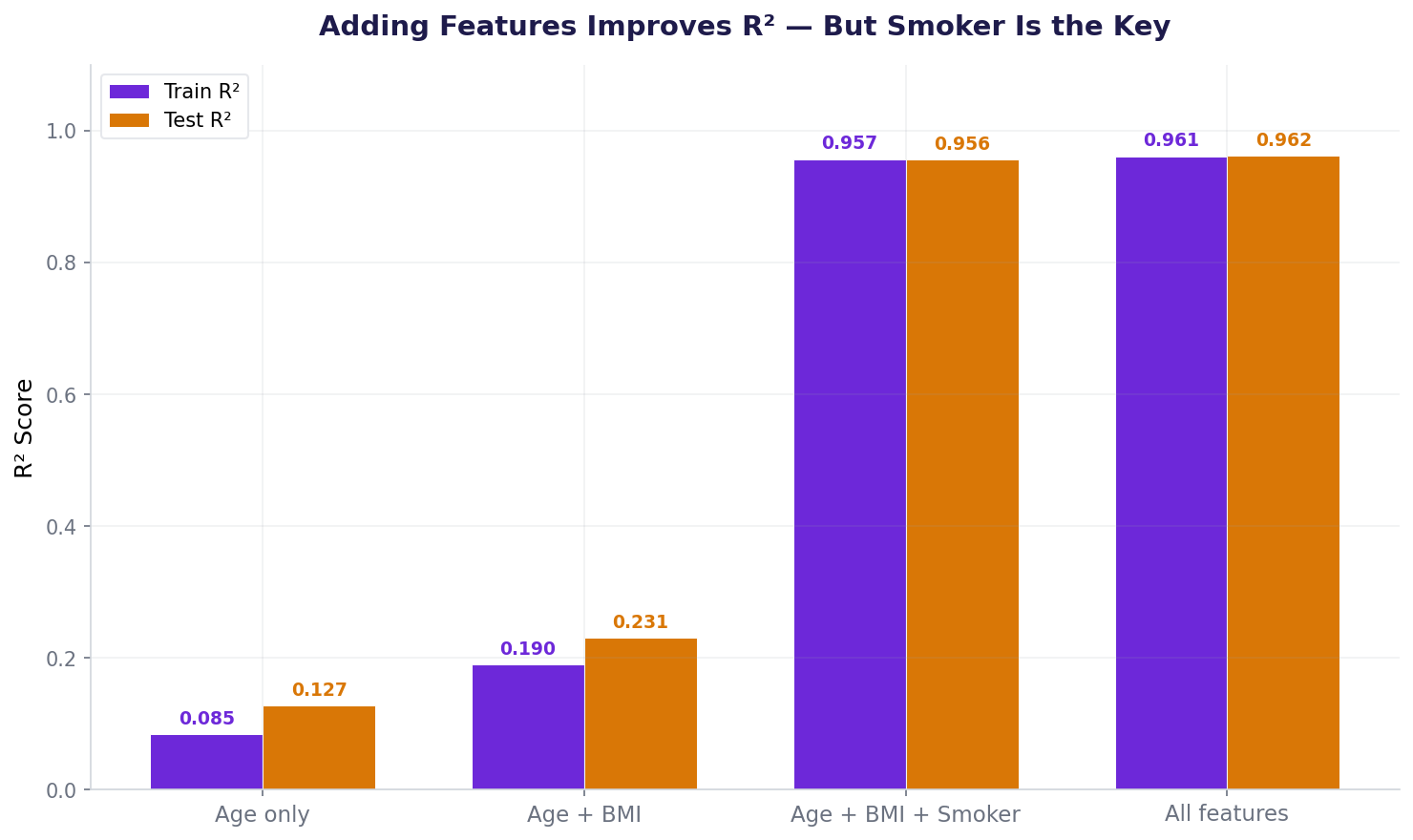
Here's the stunning result: with age and BMI alone, the best we can achieve is R²=0.24, even with degree 5 polynomial expansion. But when Arjun adds one more feature—smoker status (binary: yes/no)—watch what happens:
Wow. Adding a single binary feature is 52 percentage points better than expanding into 20 polynomial terms. This teaches the hardest lesson in machine learning: a good feature is worth more than a fancy algorithm. And when you include all features (age, BMI, smoker, children, sex, region), you hit R²=0.96 with just degree-1 (linear) terms.
Using PolynomialFeatures in sklearn
Here's how to safely use polynomial features without overfitting:
Key rules: (1) Always split before any feature engineering. (2) Fit transformers on train only. (3) Transform test with the fitted transformer. This prevents data leakage and gives honest estimates of test performance.
Multiple regression: more features, but only good ones
Multiple regression adds more original features (not transformations) to your model. With all SafeGuard features:
When you include all these features with proper encoding (smoker as 0/1, sex as 0/1, region as one-hot), linear regression (degree 1) achieves R²=0.96. No polynomial tricks needed.
Also used in...
Domain Spotlight
How AI systems use this
GPT and modern neural networks don't use polynomial features—they're too explicit. Instead, neural networks learn non-linear relationships automatically through activation functions (ReLU, sigmoid, tanh). But the principle is the same: overfitting is the enemy. That's why neural networks use dropout (randomly turning off neurons), batch normalization, and regularization (L1/L2 penalties). You're learning the same bias-variance tradeoff that powers every AI system.
Task: Train a degree-2 polynomial model on age and BMI with smoker status included. (Hint: add smoker as a numeric feature before PolynomialFeatures.) Does the test R² improve vs degree-2 without smoker? By how much? Why is the interaction term age×smoker meaningful for insurance?
Hint 1: Create a dataframe with columns: age, bmi, smoker (as 0/1)
Hint 2: Use PolynomialFeatures(degree=2).fit_transform() on all three columns
Hint 3: The interaction term age×smoker appears in the polynomial expansion. It captures: "smokers' charges accelerate with age differently than non-smokers'"
Hint 4: Compare test R² with the earlier degree-2 (age+bmi only) result: 0.2357
Interview questions: test your understanding
Quiz: 5 questions to test your knowledge
Cheatsheet: polynomial & multiple regression at a glance
| Concept | Code / Formula | Key Idea |
|---|---|---|
| PolynomialFeatures | PolynomialFeatures(degree=2) |
Adds x², x₁x₂ terms; grows fast with degree |
| Fit on train only | poly.fit_transform(X_train) |
Prevents data leakage |
| Transform test | poly.transform(X_test) |
Use fitted transformer, no new fit |
| Feature count formula | (n+d)! / (n!d!) | n=inputs, d=degree; grows exponentially |
| Overfitting sign | train R² >> test R² | Model memorized training noise |
| Sweet spot | Best test R², not best train R² | Optimal complexity for new data |
| Feature selection | Add informative features, not expansions | Good feature > many polynomial terms |
Common mistakes: what breaks and how to fix it
Key takeaways
Polynomial features seem powerful, but they're a double-edged sword.
- Polynomial expansion grows exponentially. Two features, degree 3 → 9 features. Fifty features, degree 3 → 22,100 features. Watch your feature-to-row ratio.
- Overfitting is your enemy. When train R² keeps improving but test R² drops, the model is memorizing noise. Compare test R² across degrees, not train R².
- The bias-variance tradeoff is real. Simple models underfit (high bias). Complex models overfit (high variance). The sweet spot is the test score peak.
- Feature selection beats feature engineering. A single good feature (smoker) added 52 points to R². Twenty polynomial terms added 0.01 points. Choose your features wisely.
- Always split before preprocessing. Fit transformers on train only, transform test with the fitted transformer. No leakage.
- Most real problems don't need polynomials. A linear model with the right features (lesson 6 achieved R²=0.96) beats polynomial tricks every time.
Ready to master regression at scale?
Join the Best AI Program: The AI-Era Analyst — 5 months, fully online, with placement assistance. Week 1 is free.
Explore The AI-Era Analyst →