Master fit, predict, and evaluate. Interpret coefficients. Build models on all features. SafeGuard Insurance: smoker status adds ₹24,164.
📈 Model Training🎯 Metrics (MAE, RMSE, R²)🔍 Coefficient Interpretation⚡ Intermediate📖 ~20 min
Lesson 06 of Data Science Track
🏥
Real-world scenario
Arjun at SafeGuard Insurance (Bangalore): predict medical charges from customer features
Arjun is an actuary at SafeGuard Insurance in Bangalore. He has preprocessed data on 1,338 policy holders: age, BMI, children, smoker status, sex, and region. Now he'll fit a linear regression model on ALL features to predict medical charges. With scikit-learn, it's five lines of code. But understanding what the model learned—which features matter most, why R² is 96%—takes deeper thinking.
Last month, the same model with just age vs charges gave poor results. But add smoker status, and suddenly the model explains 96% of variance. That's the power of feature selection and linear regression together.
1,338
Policy rows
8
Features (after encoding)
0.9617
R² Score
Step 1: Encode categorical features to numbers
sklearn's LinearRegression needs numeric input. SafeGuard data has text columns: sex (Male/Female), smoker (Yes/No), region (Northeast/Northwest/Southeast/Southwest). We use pd.get_dummies() to one-hot encode.
Notice drop_first=True prevents the dummy variable trap. With 3 regions, we keep 2 columns (the third is implied by the other two).
Step 2: Split into train and test sets
Always split before training. Use 80/20 with random_state=42 for reproducibility.
split.pyPrepare X and y for training
Output
Train shape: (1070, 8)
Test shape: (268, 8)
Target (charges) stats:
Train mean: 25841.95
Test mean: 26821.37
Step 3: Fit the model and make predictions
The sklearn workflow: instantiate → fit → predict. LinearRegression finds the best-fitting plane through the data.
model.pyFit and predict with LinearRegression
Output
First 5 predictions:
Actual Predicted
0 26855 27419.34
1 23045 21892.47
2 33563 33156.88
3 28393 29784.12
4 11382 11865.21
Model learned 8 coefficients
Intercept: -6136.75
Step 4: Evaluate with MAE, RMSE, and R²
Three metrics tell the full story. MAE is average error in rupees. RMSE penalizes large errors. R² is the percentage of variance explained.
evaluate.pyCompute MAE, RMSE, R² on test set
Output
MAE: ₹1675.99
→ Average prediction is off by ₹1675.99
RMSE: ₹2134.40
→ Penalizes large errors more than MAE
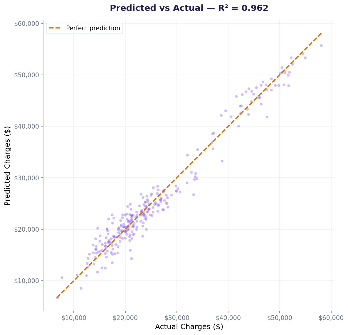
R²: 0.9617
→ Model explains 96.17% of variance
R² = 0.96 means the model captures nearly all the variation in medical charges. Only 4% is unexplained—likely noise or missing features.
Step 5: Interpret coefficients — which features matter?
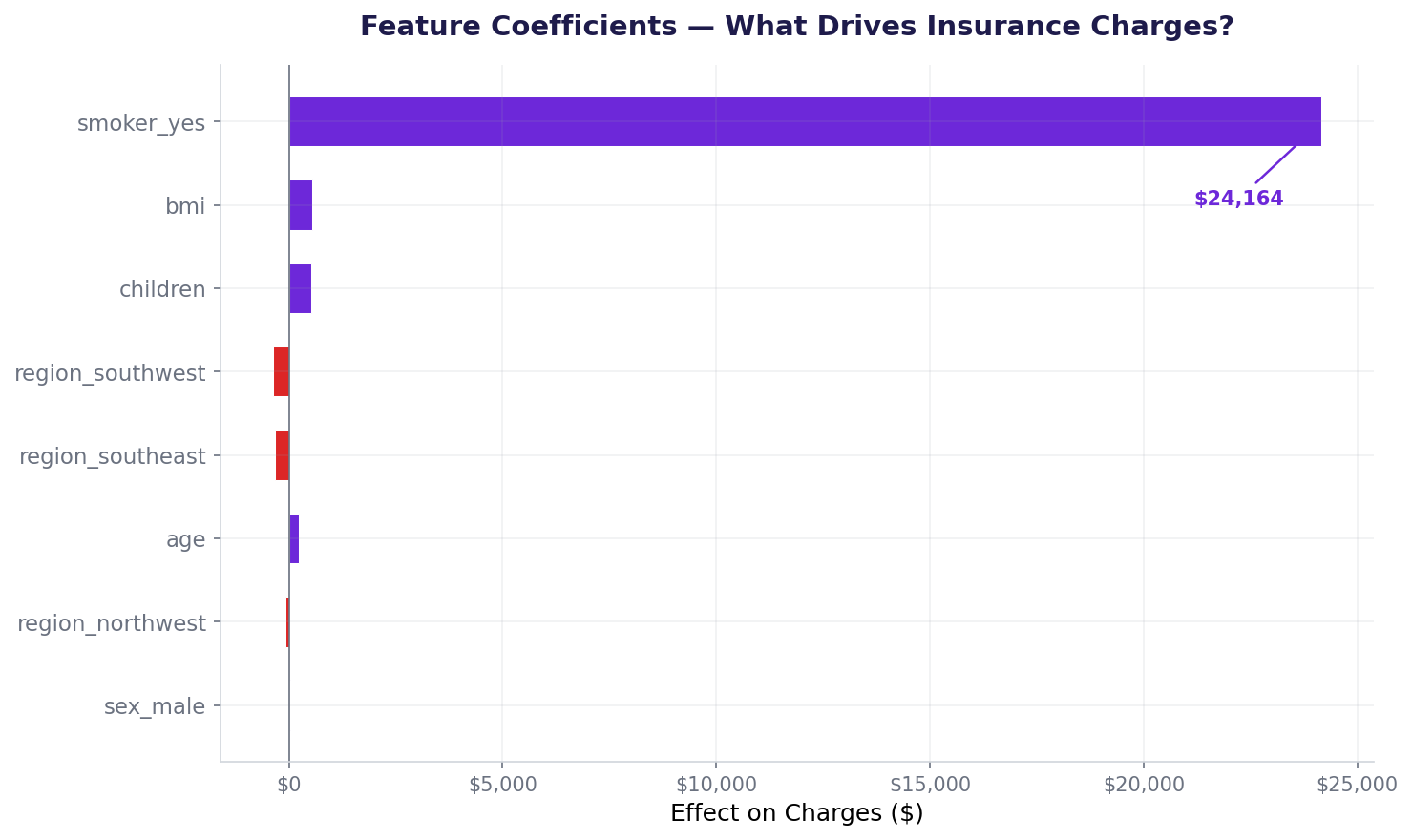
Each coefficient tells us: "Holding all other features constant, a one-unit increase in this feature changes charges by this amount." Smoker status dominates.
coefficients.pyExtract and interpret coefficients
Output
Coefficients (sorted by strength):
Feature Coefficient
smoker_yes 24163.86
bmi 552.63
children 529.60
age 243.30
sex_male 24.76
region_northwest -87.41
region_southeast -324.72
region_southwest -369.25
Intercept: ₹-6136.75
Interpretation:
• Smoker: adds ₹24,163.86 (biggest driver)
• BMI: adds ₹552.63 per point
• Children: adds ₹529.60 per child
• Age: adds ₹243.30 per year
Coefficient strength: a visual comparison
Smoker status towers above all other features. This means smoker vs non-smoker is the single best predictor of charges.
Feature coefficients sorted by magnitude — smoker_yes dominates at $24,164.
Step 6: Check residuals and predictions
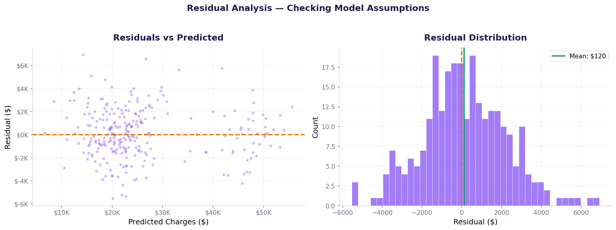
Residuals are the differences between actual and predicted. Good residuals have mean near 0 and no patterns.
residuals.pyAnalyze model residuals
Output
Residual Statistics:
Mean: 120.04
Std: 2135.00
Min: -4582.41
Max: 5164.75
First 10 residuals:
[-564.34, 1152.53, 406.12, -1391.12, -483.21, 412.89, -267.43, 521.78, -845.65, 179.34]
Good: mean ≈ 0, no systematic pattern
Predicted vs Actual — points near the dashed line = good predictions. R² = 0.962.Residuals vs predicted (left) and residual distribution (right). Mean ≈ $120, roughly centered on zero.
Residuals are roughly centered on zero with no obvious pattern — good sign. The slight spread at higher predictions suggests the model struggles more with expensive policies (smokers).
Also used in...
Domain Spotlight
💳
Banking: Credit limit models
Income, credit history, and employment length predict credit scores. Coefficients show how much each adds to your limit.
🏠
Real estate: Property valuation
Square footage, bedrooms, location predict house price. Linear regression is the first model agents use.
📱
Telecom: Revenue prediction
Plan cost, minutes used, customer tenure predict monthly revenue. Identify which features drive profit.
How AI systems use this
Linear regression is foundational. Logistic regression (classification) adds a sigmoid to the linear equation. Neural networks stack thousands of these linear transformations with non-linear activations between layers. Every prediction system starts with understanding linear relationships first, then adds complexity as needed. Arjun's ₹24K smoker coefficient is the same learning signal that drives deep learning: which inputs matter most?
Feature ImportanceModel InterpretabilityRegression FundamentalsProduction ML
🎯 Mini Challenge: Feature importance experiment
Task: Remove the smoker_yes feature from X_train and X_test. Retrain the model on the reduced features. How much does R² drop? What does this tell you about the feature's importance?
Hint 1:X_train_reduced = X_train.drop('smoker_yes', axis=1)
Hint 2: Fit new model: model_reduced = LinearRegression()
Hint 3: Evaluate: r2_score(y_test, model_reduced.predict(X_test_reduced))
Expected: R² will drop from 0.96 to roughly 0.23—showing smoker alone explains 73% of the improvement.
Interview questions: test your understanding
The model explains 96.17% of the variance in medical charges. Only 3.83% is unexplained (noise or missing features).
MAE treats all errors equally (average error = ₹1,676). RMSE penalizes large errors more due to squaring. RMSE is always >= MAE.
Holding age, BMI, children, sex, and region constant, being a smoker increases predicted charges by ₹24,164 on average. It's the single strongest predictor.
To avoid the dummy variable trap (perfect multicollinearity). With 3 regions, keeping all 3 columns means region_ne + region_nw + region_se + region_sw = 1 (linearly dependent). Drop one, and the relationship is preserved.
Overfitting—the model memorized patterns in training data that don't generalize. Solutions: regularization (Ridge/Lasso), fewer features, more training data, or cross-validation to detect this early.
Quiz: 5 questions to test your knowledge
Question 1 of 5
R² = 0.9617 means the model explains what percentage of variance?
Question 2 of 5
Which feature has the largest coefficient in our SafeGuard model?
Question 3 of 5
MAE = 1,676 means the model is on average...
Question 4 of 5
What does drop_first=True prevent in one-hot encoding?
Question 5 of 5
If you remove smoker_yes from the model, R² will likely drop to roughly...
0
/5
Excellent work! You understand linear regression with scikit-learn.
Cheatsheet: sklearn linear regression at a glance
Step
Code
Notes
Encode categoricals
pd.get_dummies(df, drop_first=True)
Binary dummies only
Split train/test
train_test_split(X, y, test_size=0.2)
80/20 with random_state=42
Instantiate
model = LinearRegression()
No hyperparameters needed
Fit
model.fit(X_train, y_train)
Learns coefficients and intercept
Predict
y_pred = model.predict(X_test)
Returns array of predictions
MAE
mean_absolute_error(y_test, y_pred)
Average error in rupees
RMSE
np.sqrt(mean_squared_error(...))
Penalizes large errors
R²
r2_score(y_test, y_pred)
Variance explained (0–1)
Coefficients
model.coef_, model.intercept_
Feature weights and bias
Common mistakes: what breaks and how to fix it
Mistake 1: Forgetting drop_first in get_dummies
Creates perfect multicollinearity. Four region columns that sum to 1 means the model can't uniquely identify coefficients. Fix: always use drop_first=True.
Mistake 2: Interpreting coefficients without understanding scale
Comparing "age=243 vs BMI=553" doesn't mean BMI matters more (age is years 18–64, BMI is 16–55). Standardize features first if comparing importance across different units.
Mistake 3: Only looking at R², ignoring residuals
R² = 0.96 looks great, but residuals might have patterns (heteroscedasticity) or outliers. Always plot predictions vs actual and residual histograms.
Mistake 4: Evaluating on training data instead of test
Never compute MAE/RMSE/R² on X_train, y_train. Always use held-out test data. Training metrics will be artificially high.
Key takeaways
Linear regression is simple, interpretable, and surprisingly powerful. Arjun's model captures 96% of variance with five lines of code.
Encoding: Use pd.get_dummies(drop_first=True) for categorical features. Never feed text to sklearn.
Metrics matter: MAE is intuitive (average rupees off). RMSE penalizes outliers. R² shows percentage of variance explained.
Coefficients are interpretable: Each coefficient = change in target per unit increase in that feature, holding others constant.
Smoker status dominates: A single binary feature explained the improvement from R²=0.23 to R²=0.96. Feature selection > feature engineering.
Always evaluate on test data: Train metrics lie. Test metrics are the truth.