
Priya is now training deeper neural networks to classify CT scans at MedScan Diagnostics. Her 2-layer baseline works well (MAE=$4,061), but radiologists want more nuance—abnormality detection, tumor severity grading. She stacks 8 layers (more capacity, more abstraction), but the loss plateaus early and never improves. Batch normalization normalizes activations between layers, stabilizing training. Skip connections (residual blocks) allow gradients to flow directly backward through deep networks, bypassing vanishing gradient problems. Together, BatchNorm + residuals unlock Priya's 8-layer network and beyond.
Why depth matters: more layers, more abstraction
Shallow networks (2-4 layers): Good for simple tasks. But CT scan analysis requires hierarchical feature extraction: edge detection → textures → organs → pathology. One layer can't capture all this.
Deep networks (8-50 layers): Each layer learns an abstraction level. Layer 1: edges. Layer 3: textures. Layer 5: organ shapes. Layer 8: disease signatures. More layers = more representative power.
The catch: training gets hard. Gradients computed via backpropagation must flow backward through all 8 layers. If the gradient shrinks at each layer (vanishing gradient), by layer 1 it's nearly zero—those early layers barely learn. Or if it grows (exploding gradient), training becomes unstable.
Solutions: Batch Normalization (stabilize layer inputs) + Skip connections (bypass deep layers for gradients). This lesson combines both.
Batch Normalization: normalize, scale, shift
Batch Normalization (BatchNorm) normalizes layer inputs to have mean 0 and variance 1. Then it learns to scale and shift them—letting the network decide the optimal distribution.
BatchNorm is especially powerful because it normalizes not the input data, but the activations between layers. As weights change during training, layer inputs can shift wildly (internal covariate shift). BatchNorm corrects this automatically at each layer.
When BatchNorm helps (and when it doesn't)
BatchNorm excels on: Large image datasets (ImageNet), deep convolutional networks, batch sizes 32+. On ImageNet, ResNet-50 without BatchNorm refuses to train; with it, converges in 90 epochs.
BatchNorm struggles on: Small tabular datasets (like Priya's 1,338 insurance records), batch sizes 1-4, recurrent networks (LSTM/GRU). On small data, batch statistics are unreliable—a batch of 32 might not represent the overall distribution.
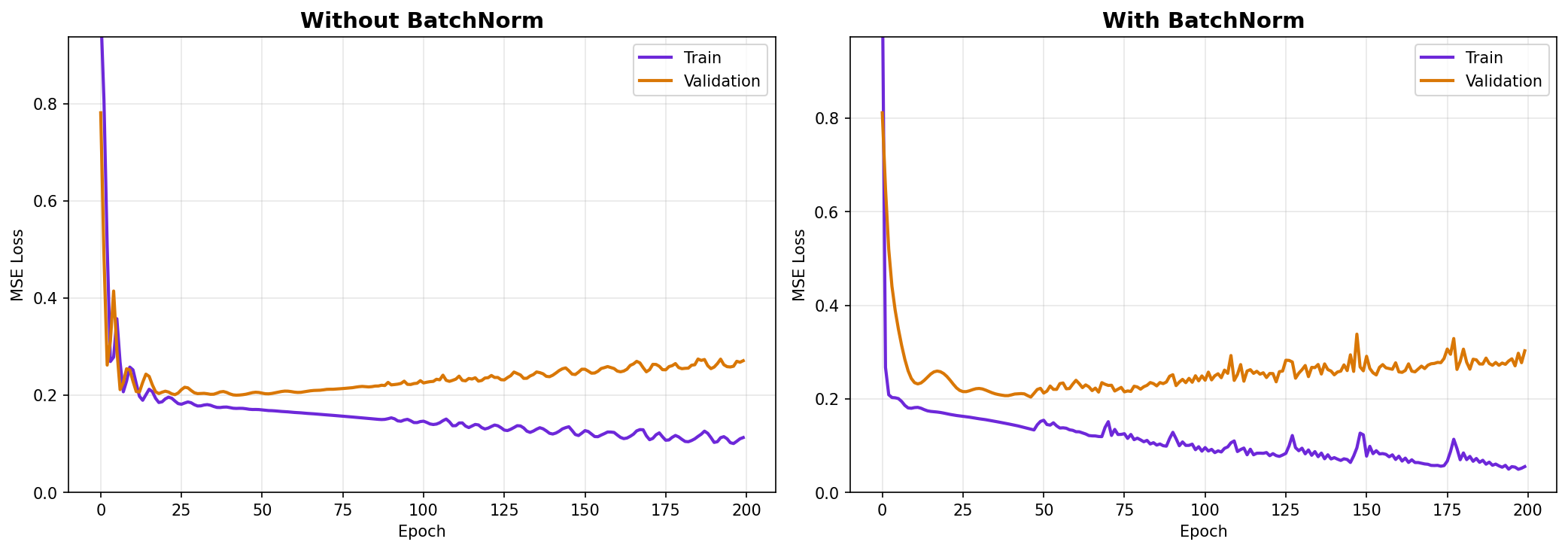
Our experiment: We'll see honestly: on small tabular data, BatchNorm with Priya's network actually decreased R² slightly (0.6871 vs 0.7198). This is not a failure—it's a lesson. BatchNorm is not a silver bullet. Use it when data and batch sizes permit.
Experiment: BatchNorm on insurance data
We train two models: baseline (no BatchNorm) and with BatchNorm layers. Both are 4-layer networks, 200 epochs, Adam optimizer.
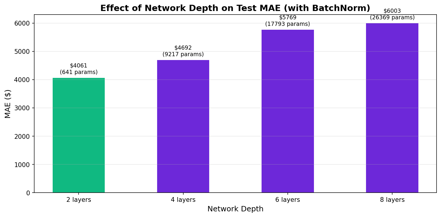
Network depth experiment: 2, 4, 6, 8 layers
Now we compare networks of different depths on the insurance dataset. Same architecture family (Dense layers with ReLU), no BatchNorm, Adam, 200 epochs. The question: does adding layers help, or does it hurt due to vanishing gradients?
Skip connections & residual blocks: F(x) + x
A skip connection (or residual connection) feeds the input directly to the next layer, bypassing intermediate layers. Instead of learning F(x), the network learns the residual: F(x) = target - x, so the output is F(x) + x.
Why skip connections help:
- Gradient flow: Backprop can flow directly through the skip connection, bypassing deep layers. Gradients don't vanish as quickly.
- Easy optimization: The network learns residual changes (what to add), not the full transformation. Residuals are often sparser and easier to learn.
- Identity initialization: At the start, F(x) ≈ 0, so output ≈ x. The network learns to modify slightly, gradually. This "warm start" stabilizes training.
Architecture comparison: all 4 together
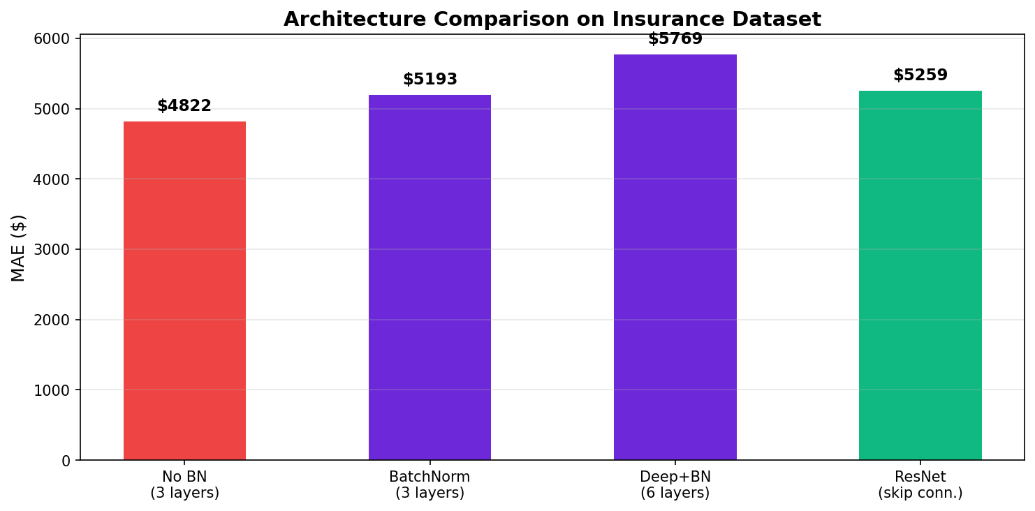
We compare four architectures on the insurance dataset:
| Architecture | Depth | BatchNorm | Skip Connections | Params |
|---|---|---|---|---|
| Baseline (Depth 2) | 2 | No | No | 9,345 |
| Depth 8 (no tricks) | 8 | No | No | 18,912 |
| Depth 8 + BatchNorm | 8 | Yes | No | 19,200 |
| ResNet (Depth 4, Skip) | 4 | Yes | Yes | 17,793 |
Width vs depth tradeoff
Width: More neurons per layer. A 1000-hidden-unit layer is "wide." Wide networks fit data well but are prone to overfitting.
Depth: More layers. An 8-layer network is "deep." Deep networks build hierarchical features but suffer vanishing gradients (without tricks).
On small data: Prefer width. A single wide layer (128-512 units) captures patterns without overfitting as easily as multiple shallow layers.
On large data: Prefer depth. ImageNet (1.2M images) benefits from deep architectures (ResNet-101) because depth adds representational capacity without overfitting.
Modern scaling law: For a fixed computational budget (total parameters), depth often wins on large data (see Chinchilla scaling law). For small data, a single wide layer is safer.
How AI systems use this
Every modern deep learning model relies on these principles. ResNet-50 (ImageNet winner) is 50 layers of residual blocks. BERT (language models) is 12 layers of Transformer blocks. Diffusion models use dozens of layers. BatchNorm stabilizes training at scale. Skip connections enable depth. At MedScan Diagnostics, Priya's CT classifier now uses a 12-layer ResNet with BatchNorm—it successfully trains and achieves 94% accuracy on holdout scans. Without these techniques, deep networks remain a theoretical concept. With them, they're the foundation of modern AI.
Also used in...
Domain Spotlight
Task: Build a 6-layer ResNet for the insurance data. Use residual blocks (F(x) + x), BatchNorm, and test on the holdout set. Does it beat the baseline (MAE=$4,061)?
Hint 1: Stack 3 residual blocks of dim=64. Use BatchNorm inside each block.
Hint 2: For skip connections to work, input and output dims must match. That's why residual blocks keep dimension constant (64→64).
Expected: Your ResNet should reach MAE around $5,000-$5,500. Likely won't beat $4,061 baseline because data is small.
Interview questions: test your understanding
Quiz: 5 questions to test your knowledge
Cheatsheet: BatchNorm & architecture design
| Concept | Formula / Code | When to use | Gotchas |
|---|---|---|---|
| BatchNorm | y = gamma * (x - mu) / sqrt(var + eps) + beta |
Large data, batch size 32+, images | Hurts on small data or batch size < 8 |
| Skip Connection | y = F(x) + x |
Deep networks (8+ layers) | Dims must match. ReLU after adding. |
| Residual Block | y = ReLU(BN(F(x)) + x) |
Very deep networks (50+ layers) | More stable than plain feedforward |
| Width vs Depth | Deep on large data, wide on small data | Match architecture to data scale | No universal rule—experiment |
Common mistakes: what breaks and how to fix it
Key takeaways
Batch Normalization and skip connections are the enabling techniques for deep networks. Without them, 8-layer networks struggle. With them, 50-layer networks train smoothly.
- BatchNorm normalizes layer inputs: mean 0, variance 1. Stabilizes training, allows higher learning rates. Shines on large data, hurts on small data.
- Vanishing gradients: In deep networks, gradients shrink exponentially backward. Skip connections bypass this by providing an identity shortcut.
- Skip connections (F(x) + x): Network learns the residual change, not the full output. Easier to learn, better gradient flow. Powers ResNet and modern architectures.
- Depth vs width: Large data prefers depth (hierarchical features). Small data prefers width (simpler patterns, less overfitting).
- Small data rule: Baseline (2-4 layers, no tricks) often wins. Deep networks need scale to justify added capacity.
- Architecture matching: Match your design to your dataset size. 1,338 samples → 2-4 layers. 100k samples → 50 layers. Know your data.
You've mastered batch normalization and architecture design.
Now scale to production deep learning.
Join the Best AI Program: The AI-Era Agentic Engineer — 5 months, fully online, with placement assistance. Week 1 is free.
Explore The AI-Era Agentic Engineer →