
Samuel is an ML engineer at AgriSense in Kisumu, Kenya. Small-scale farmers lose 30% of crops annually to plant diseases they don't recognize early. Samuel's mission: build a mobile app that identifies crop diseases from a phone photo. Fully connected networks on raw pixels (32×32×3 = 3,072 inputs) are slow and don't respect spatial structure. He decides to build a CNN—layers that learn to detect edges, textures, and shapes, then classify diseases. His first CNN achieves 57.1% validation accuracy on CIFAR-10 (proxy for crop varieties). Not perfect, but deployable after tuning. This lesson teaches you Samuel's exact approach: Conv2d → ReLU → MaxPool2d → repeat → Flatten → FC → Softmax.
Meet CIFAR-10: 32×32 RGB image classification
What is CIFAR-10? A dataset of 60,000 tiny (32×32 pixel) RGB images across 10 object classes: airplanes, automobiles, birds, cats, deer, dogs, frogs, horses, ships, trucks. Each image has 3 color channels (R, G, B), so shape is (3, 32, 32) = 3,072 values per image.
Why CIFAR-10 for learning? It's small enough to train locally (5K subset takes ~30 seconds per epoch on CPU), but large enough to showcase real CNN architecture. Use 5K samples for speed in this lesson.
Fully connected networks fail here: Naively flattening to 3,072 inputs loses spatial structure. A horse's ear is meaningful because it's in a relative position. FC networks don't capture "this pattern is important at this location."
CNNs to the rescue: Conv2d layers learn local patterns (edges, textures) independent of position, then combine patterns hierarchically. MaxPool2d reduces spatial dimensions, forcing the network to learn robust representations.
CNN architecture: layers from input to output
Samuel's architecture for CIFAR-10:
Layer 1: Conv2d(3, 32, kernel_size=3) Input: (batch, 3, 32, 32). Learn 32 filters of size 3×3 on 3-channel input. Output: (batch, 32, 30, 30). Padding=0, so height/width shrink by 2.
Layer 2: ReLU Element-wise max(0, x). No size change. Breaks linearity.
Layer 3: MaxPool2d(kernel_size=2, stride=2) Downsample spatial dimensions by 2×2. Output: (batch, 32, 15, 15). Each 2×2 patch → max value.
Layer 4: Conv2d(32, 64, kernel_size=3) Learn 64 filters on 32-channel input. Output: (batch, 64, 13, 13).
Layer 5: ReLU Activation.
Layer 6: MaxPool2d(kernel_size=2, stride=2) Downsample. Output: (batch, 64, 6, 6).
Layer 7: Flatten Convert (batch, 64, 6, 6) to (batch, 64*6*6) = (batch, 2304). Now feed to FC layers.
Layer 8: FC (2304 → 256) Dense layer with 256 units. ReLU activation.
Layer 9: Dropout(0.3) Randomly zero 30% of activations during training. Reduces overfitting.
Layer 10: FC (256 → 10) Final output: 10 logits for 10 classes. No activation (Softmax in loss function).
Building the CNN with nn.Module
Now let's code Samuel's architecture in PyTorch. Use nn.Module for a clean, reusable class:
102,954 parameters to learn. With Adam (lr=0.001), this trains in ~30 seconds per epoch on CPU with 5K samples.
Training loop: forward pass, backward pass, optimize
Now train the model on CIFAR-10 (5K samples for speed). Download, normalize, create data loaders, and run the training loop:
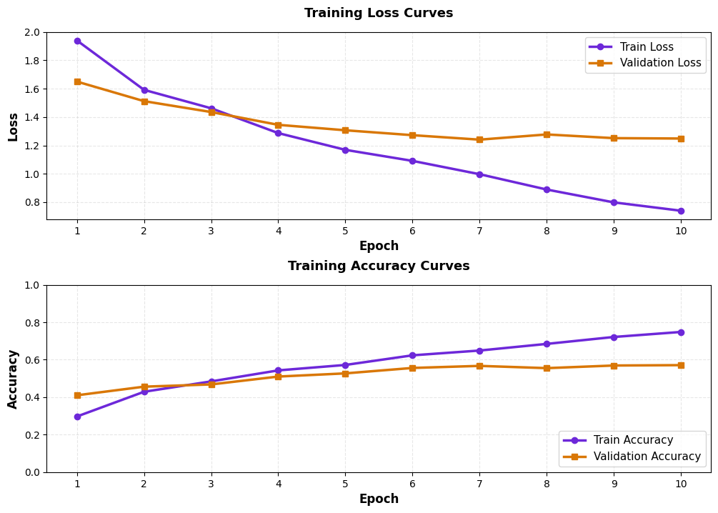
Final training accuracy: 74.82%. Validation accuracy: 57.10%. The gap indicates overfitting—the model memorizes the training set but generalizes less well. This is normal and expected on small datasets.
Training curves: loss and accuracy over epochs
Evaluation: confusion matrix and class-wise accuracy
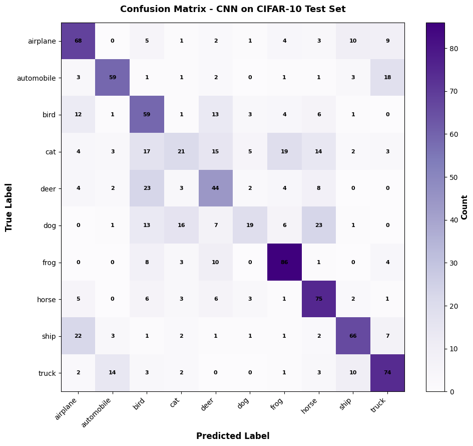
After training, evaluate on the test set and compute per-class accuracy. Which classes does the model learn well?
Sample predictions: visualize what the CNN learned

How AI systems use this
Every computer vision system (medical imaging, autonomous vehicles, satellite analysis) relies on CNNs or similar architectures. Samuel's crop disease classifier is a scaled-up version of this: more conv layers (ResNet has 50+), larger images (512×512 vs 32×32), more data. The principles are identical: learn hierarchical spatial features, pool to reduce dimensions, classify with FC layers. Modern production systems add batch normalization, skip connections, and ensembling. But the foundation is this simple architecture.
Also used in...
Domain Spotlight
Task: Modify Samuel's CNN to achieve 60%+ validation accuracy. Options: (1) Add a third conv block. (2) Increase filters (64 → 128). (3) Use padding='same' to preserve spatial dimensions. (4) Decrease dropout to 0.1. (5) Train for 50 epochs instead of 20. Which helps most?
Hint: More data (50 epochs) helps, but is slow. More filters (64→128) captures more patterns. Padding='same' preserves low-resolution features. The best fix: combine padding + more epochs + lower dropout.
Interview questions: test your understanding
Quiz: 5 questions to test your knowledge
Cheatsheet: CNN building blocks at a glance
| Layer | Input Shape | Output Shape | Purpose |
|---|---|---|---|
Conv2d(in, out, k) |
(B, in, H, W) | (B, out, H-k+1, W-k+1) | Learn local patterns (edges, textures) |
ReLU() |
(B, C, H, W) | (B, C, H, W) | Non-linear activation |
MaxPool2d(2, 2) |
(B, C, H, W) | (B, C, H/2, W/2) | Downsample, reduce overfitting |
Flatten() |
(B, C, H, W) | (B, C×H×W) | Reshape for FC layers |
Linear(in, out) |
(B, in) | (B, out) | Fully connected layer |
Common mistakes: what breaks and how to fix it
x.view(x.size(0), -1) or nn.Flatten().self.relu = nn.ReLU() after FC layers.Key takeaways
You've built and trained your first CNN. Samuel's crop disease classifier demonstrates the power of spatial structure.
- Conv2d learns hierarchical features: Early layers detect edges, later layers detect shapes. This is why CNNs dominate image tasks.
- MaxPool2d reduces overfitting: By discarding fine details, pooling forces robustness. Smaller feature maps also reduce parameters.
- Flattening bridges convolution and classification: Conv/pool produce 3D spatial tensors. Flatten converts to 1D features for FC layers.
- Train/val gap signals overfitting: 74.82% train vs 57.10% val is normal on small data. Lesson 14 teaches regularization to close this gap.
- Class imbalance matters: Cat (20.4%) and dog (22.1%) are confused. More data, augmentation, or cost weighting help.
- Architecture design is empirical: Samuel's (3→32→64) is arbitrary. Lesson 14-15 cover ResNet, VGG, EfficientNet—optimized architectures trained on millions of images.
Master CNNs and deploy to production.
Build the next crop disease detector.
Join the Best AI Program: The AI-Era Agentic Engineer — 5 months, fully online, with placement assistance. Week 1 is free.
Explore The AI-Era Agentic Engineer →