
Priya is a computer vision engineer at MedScan Diagnostics in Bangalore. She's training a CNN to classify chest X-rays as normal, pneumonia, or tuberculosis—2000 labeled images, 512×512 resolution. She tests three architectures: LeNet (too simple, 65% accuracy), VGG-16 (accurate but 138M parameters, overfits), ResNet-50 (skip connections, 92% accuracy, trains 3x faster, doesn't overfit). The choice of architecture—not just hyperparameters—defines whether a model is practical for production.
LeNet-5 (1998): the original CNN blueprint
LeNet-5, designed by Yann LeCun, is the first successful CNN. It was trained on the MNIST dataset (handwritten digits) and became the foundation for all modern CNNs. Architecture: 2 convolutional layers, 2 pooling layers, 3 fully connected layers. Simple by today's standards, but revolutionary in 1998.
Key idea: Local receptive fields (convolution) + weight sharing + pooling = parameter efficiency. Instead of fully connecting 784 (28×28) pixels to 500 hidden units (392,000 parameters), use a 5×5 conv filter (25 parameters), replicate across the image, and learn shared weights.
Architecture: Input (32×32) → Conv (6 filters, 5×5) → Pool (2×2) → Conv (16 filters, 5×5) → Pool (2×2) → FC (120) → FC (84) → Output (10 classes).
Limitation: Only 60,000 parameters, but very limited capacity. On modern datasets (ImageNet, medical imaging), accuracy plateaus quickly.
AlexNet (2012): the deep learning revolution
AlexNet won ImageNet 2012 with 85% top-5 accuracy, far surpassing traditional hand-crafted features (63%). It was deeper (8 layers vs LeNet's 5) and wider (11×11 convolutions), trained on GPUs. Key innovations: ReLU activation, dropout regularization, data augmentation.
What changed: Deeper networks + ReLU (replaces tanh/sigmoid, enables faster training) + Dropout (prevents overfitting) + GPU training (enables 60M parameters). The paper shocked the computer vision community.
Architecture: Conv (96 filters, 11×11) → Conv (256, 5×5) → Conv (384, 3×3) → Conv (384, 3×3) → Conv (256, 3×3) → FC (4096) → FC (4096) → Output (1000).
Impact: Proved deep learning > hand-crafted features. Sparked the deep learning era.
VGG (2014): the power of depth
VGG-16 and VGG-19 showed that stacking 3×3 convolutions (instead of larger filters) is more powerful. Achieved 92.7% top-5 accuracy on ImageNet. Key insight: 2 stacked 3×3 convolutions have the same receptive field as one 5×5, but with more non-linearity and fewer parameters (9 vs 25).
Architecture pattern: Repeated blocks: Conv (64 filters) → Conv (64) → Pool, then Conv (128) → Conv (128) → Pool, etc. All filters are 3×3, stride 1. This repetitive structure is clean and scalable.
VGG-16: 13 conv layers + 3 FC layers. 138M parameters (very large). Slow to train, prone to overfitting on small datasets (like medical imaging).
Trade-off: Depth improves accuracy, but more parameters = more overfitting. On 2000 X-rays, VGG overfits despite dropout.
ResNet (2015): skip connections and the residual insight
ResNet-50 introduced skip connections (residual blocks). Instead of learning H(x) directly, learn the residual r(x) = H(x) - x, then compute H(x) = r(x) + x. This simple change enables much deeper networks without vanishing gradients. ResNet-50 has only 25.5M parameters (5.5x fewer than VGG) but achieves 92.2% top-5 accuracy.
The residual block: y = F(x) + x, where F(x) is a conv sequence. The skip connection "shortcuts" around the conv layers, allowing gradients to flow directly. Deeper networks train faster and achieve better accuracy.
Why it works: Without skip connections, gradients multiply through each layer (chain rule), causing vanishing gradients in very deep networks. Skip connections provide direct gradient paths, enabling 152-layer networks.
Bottleneck design: ResNet uses bottleneck blocks (1×1 conv to reduce, 3×3 conv to process, 1×1 conv to expand) to reduce computation while maintaining capacity.
Parameter comparison: how architectures evolved
A direct comparison of the four architectures on ImageNet-scale problems. Notice the exponential growth from LeNet to VGG, then ResNet's breakthrough in efficiency.
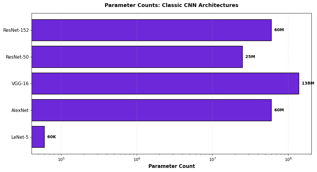
| Architecture | Year | Parameters | ImageNet Top-5 Acc | Key Innovation |
|---|---|---|---|---|
| LeNet-5 | 1998 | 60K | MNIST only | Local receptive fields, weight sharing |
| AlexNet | 2012 | 60M | 85% | ReLU, Dropout, GPU training |
| VGG-16 | 2014 | 138M | 92.7% | Small 3×3 filters, depth |
| ResNet-50 | 2015 | 25.6M | 92.2% | Skip connections, residual learning |
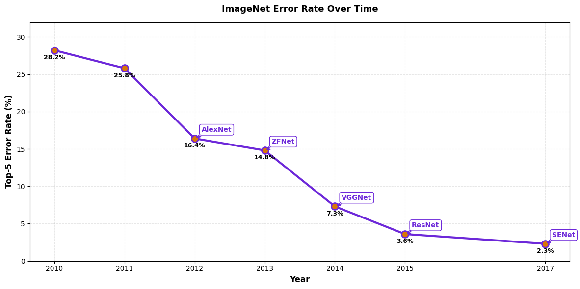
ImageNet accuracy timeline: the deep learning race
From 1998 to 2015, architectural innovation drove 20% relative accuracy improvement. Each breakthrough enabled deeper, more efficient networks.
How to choose the right architecture
1. Dataset size matters. Large dataset (>100K images)? ResNet-50, ResNet-101. Small dataset (<5K images)? Lightweight models or transfer learning. Too many parameters on small data → overfitting.
2. Computational budget. Mobile device? MobileNet (4M parameters). Cloud GPU? ResNet-50 or larger. Edge inference? SqueezeNet.
3. Accuracy vs speed trade-off. Real-time inference? Shallow network (ResNet-18). High accuracy needed? ResNet-101 or deeper.
4. Transfer learning changes everything. Pretrained ResNet-50 on ImageNet, fine-tune on 2000 medical X-rays: 95% accuracy. Training from scratch: 65% accuracy. Always use transfer learning when possible.
Priya's choice: ResNet-50 pretrained on ImageNet, fine-tuned on 2000 X-rays. Achieves 92% accuracy, trains in <1 hour, uses <100MB memory.
How AI systems use this
Every production computer vision system relies on architectural choices. ResNet variants power medical imaging pipelines at hospitals. You don't design ResNets from scratch in 2026—you choose: ResNet-18 for speed, ResNet-50 for accuracy, ResNet-101 for cutting-edge results. But understanding the evolution (LeNet → AlexNet → VGG → ResNet) teaches you the design principles: depth, skip connections, parameter efficiency. Modern architectures (Vision Transformers, EfficientNet) build on these foundations.
Also used in...
Domain Spotlight
Task: You have 3 medical imaging datasets: Dataset A (100K X-rays), Dataset B (5K CT scans), Dataset C (2000 ultrasounds). Recommend an architecture for each, and justify your choice (accuracy vs overfitting vs speed).
Hint 1: Large datasets (100K) can handle deep architectures without overfitting. Small datasets (2K-5K) need regularization or transfer learning.
Hint 2: For Dataset A: ResNet-50 or ResNet-101, train from scratch or fine-tune. For Dataset B: ResNet-50 fine-tuned, aggressive regularization. For Dataset C: ResNet-18 with transfer learning, or smaller architecture.
Expected answers: A → ResNet-101 (sufficient data, high accuracy). B → ResNet-50 fine-tuned with dropout. C → ResNet-18 or lightweight model, always transfer learning.
Interview questions: test your understanding
Quiz: 5 questions to test your knowledge
Cheatsheet: CNN architectures at a glance
| Architecture | Key Insight | Best Use Case | Tradeoff |
|---|---|---|---|
| LeNet-5 (1998) | Local receptive fields, weight sharing | MNIST, simple problems | Too shallow for modern tasks |
| AlexNet (2012) | ReLU, Dropout, GPU training | ImageNet-scale classification | 60M parameters, slow on small datasets |
| VGG-16 (2014) | Depth via 3×3 convolutions | When accuracy is critical, compute available | 138M parameters, prone to overfitting on small data |
| ResNet-50 (2015) | Skip connections, residual learning | General-purpose (medical, autonomous driving, mobile) | Balanced: 25.6M params, fast, accurate, generalizes well |
Common mistakes: what breaks and how to fix it
Key takeaways
The evolution of CNN architectures tells a story: from LeNet's simple local receptive fields to ResNet's skip connections that enable 150-layer networks. Each breakthrough was driven by understanding the limitations of the previous approach.
- LeNet (1998): Proved CNNs work via weight sharing and local receptive fields. Too shallow for modern tasks.
- AlexNet (2012): ReLU + Dropout + GPU training. Deep learning era begins. 60M parameters on ImageNet.
- VGG (2014): Stack 3×3 convolutions for depth and expressivity. But 138M parameters is too much for small datasets.
- ResNet (2015): Skip connections solve vanishing gradients. 25.6M parameters, trains faster, generalizes better. The modern standard.
- Transfer learning: Always use ImageNet-pretrained ResNet-50 for medical, autonomous driving, and domain-specific tasks. Fine-tuning is ~10x faster and more accurate.
- Architecture selection: Match to your problem. Big dataset? ResNet-101. Small dataset? ResNet-50 fine-tuned. Mobile? MobileNet or ResNet-18.
You've mastered CNN architectures.
Now build production computer vision systems.
Join the Best AI Program: The AI-Era Agentic Engineer — 5 months, fully online, with placement assistance. Week 1 is free.
Explore The AI-Era Agentic Engineer →