
Last lesson, Aisha built a single perceptron—a linear decision boundary. But medical charge prediction isn't linear. A single neuron can't capture the complex relationships: how age, BMI, smoker status, and region combine to determine charges. This lesson, she builds her first true neural network: 3 hidden layers (64, 32, 1 neurons) that learn non-linear transformations of her features. Her R² jumps from 0.941 to 0.9575. This is the leap from rules to learning.
By the end, Aisha can predict charges for any customer profile and explain how the network learned to spot complex patterns in the data. She's no longer writing rules; the network writes them.
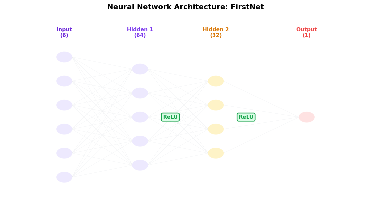
Architecture of FirstNet — the network design
How the layers connect
Input layer (6 neurons): age, bmi, smoker, region, children, sex — raw features from insurance data.
Hidden layer 1 (64 neurons): each neuron is a weighted combination of all 6 inputs, passed through ReLU activation. It learns initial charge patterns: "if age is high and smoker is yes, charge goes up." 6×64 = 384 weights + 64 biases = 448 parameters.
Hidden layer 2 (32 neurons): receives 64 outputs from layer 1, learns to combine those patterns. 64×32 = 2,048 weights + 32 biases = 2,080 parameters. Dimension reduction (64→32) is deliberate—learns a compressed representation.
Output layer (1 neuron): final prediction of charges. 32×1 = 32 weights + 1 bias = 33 parameters. No activation function (we want unbounded regression, not 0-1 range).
Total: 448 + 2,080 + 33 = 2,561 parameters. Each one learned during training.
Why this architecture?
Layer 1 (64 units): Learns basic feature combinations. One neuron might learn "smoker_yes + high_age → high_charge". Another learns "high_bmi → moderate_charge". 64 neurons capture many such patterns in parallel.
Layer 2 (32 units): Combines patterns from layer 1. Learns higher-level abstractions: "smoker + age both high → very high charge". The dimension reduction (64→32) is a bottleneck—forces the network to compress information, learning only the most important patterns.
No BatchNorm or Dropout yet: For this lesson, we keep it simple. ReLU activation is fast and avoids vanishing gradients (where gradients approach zero). No output activation because regression targets are unbounded (charges can be $5k–$50k).
Depth > Width: 3 layers with 64→32→1 neurons work better than a single wide layer (e.g., 6→128→1). Depth allows learning hierarchical, multi-step transformations.
Step 1: Define the network architecture
We inherit from nn.Module and define layers in __init__, then the forward pass in forward().
Step 2: Define loss function and optimizer
MSE (Mean Squared Error) measures prediction error. Adam optimizer updates weights using adaptive learning rates—smart, fast convergence.
Step 3: Prepare data with DataLoader
Batching speeds up training and stabilizes gradients. 32 samples per batch is standard for insurance data (1,338 samples = ~42 batches per epoch).
Step 4: Training loop — learn weights over 100 epochs
For each epoch: (1) iterate through batches, (2) forward pass, (3) compute loss, (4) backward pass (compute gradients), (5) optimizer.step() (update weights). Also compute validation loss.
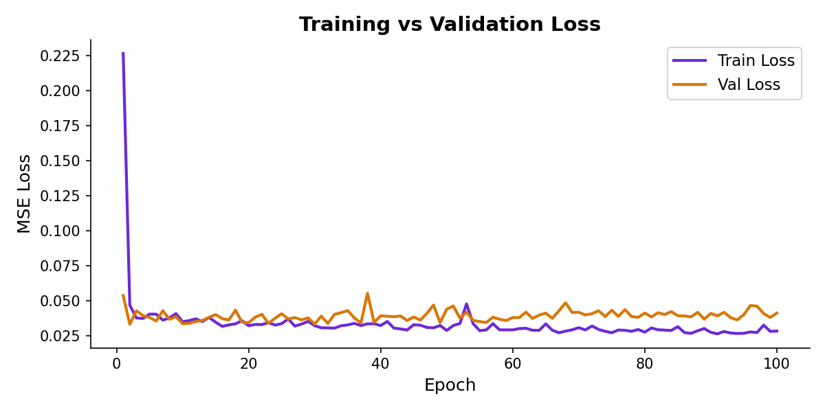
Training dynamics — what's happening under the hood?
Training loss decreases steadily (network learning patterns). Validation loss improves until epoch 25, then plateaus—an early stopping signal.
Step 5: Unscale predictions for business metrics
The model learned on scaled targets (mean=0, std=1). To report in dollars, we reverse the scaling.
Step 6: Make a prediction — Arjun's profile
Arjun is 35 years old, BMI 22.5, non-smoker, 0 children. What will his annual charges be?
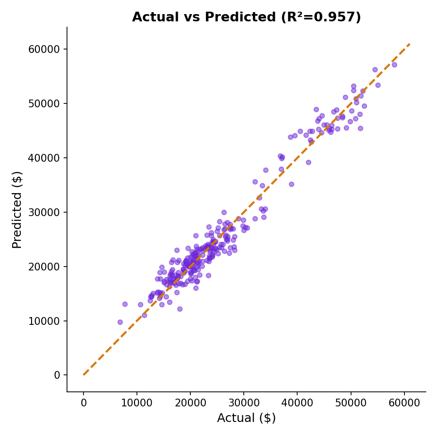
Actual vs predicted — how good are our forecasts?
Points close to the dashed line (perfect prediction) = good. Scattered widely = high error. Our R² = 0.9575 means 95.75% of variance is captured.
How AI systems use this
FirstNet is a foundation. This architecture—input → hidden layers → output—is used everywhere: image classification (conv layers instead of linear), NLP (transformers instead of ReLU), recommendation systems. The only difference is the activation function and layer type. The principle is always the same: learn hierarchical, non-linear transformations of data. Aisha's 3-layer network predicts charges; Google's BERT uses 24 layers to predict the next word. Same idea, different scale.
Also used in...
Domain Spotlight
Task: Modify FirstNet to add BatchNorm after layer 1 and Dropout (p=0.2) after layer 2. Why would these help? Train for 50 epochs and compare validation loss to the original.
Hint 1: Import: from torch.nn import BatchNorm1d, Dropout
Hint 2: In __init__: self.bn1 = BatchNorm1d(64) and self.drop = Dropout(p=0.2)
Hint 3: In forward(): x = self.bn1(torch.relu(self.fc1(x))) and x = self.drop(torch.relu(self.fc2(x)))
Hint 4: Remember to call model.train() during training and model.eval() during validation.
Expected: Validation loss should be slightly lower due to better regularization and stabilized gradients.
Interview questions: test your understanding
Quiz: 5 questions to test your knowledge
Cheatsheet: PyTorch neural networks at a glance
| Component | Syntax | Purpose |
|---|---|---|
| Define layer | nn.Linear(in, out) |
Fully connected layer with weights and biases |
| ReLU activation | torch.relu(x) |
Non-linearity: max(0, x) — no vanishing gradients |
| Loss function | nn.MSELoss() |
Mean squared error for regression targets |
| Optimizer | torch.optim.Adam(model.parameters(), lr=0.01) |
Adaptive learning rate, combines momentum + RMSprop |
| DataLoader | DataLoader(dataset, batch_size=32) |
Batching for efficient mini-batch gradient descent |
| Train mode | model.train() |
Enable dropout and batchnorm updates |
| Eval mode | model.eval() |
Disable dropout, use running stats for batchnorm |
| Backward pass | loss.backward() |
Compute gradients via backpropagation |
| Update weights | optimizer.step() |
Apply gradient updates to weights |
Common mistakes: what breaks and how to fix it
model.eval() means dropout is still active (zeros neurons), and batchnorm uses batch statistics instead of running statistics. Validation metrics will be artificially low.You've built your first neural network.
Now train it on real-world production data.
Join the Best AI Program: The AI-Era Agentic Engineer — 5 months, fully online, with placement assistance. Week 1 is free.
Explore The AI-Era Agentic Engineer →