Master generative models: VAE for generation, GANs with adversarial training, diffusion models, and comparing architectures. Create synthetic medical images.
GAN • Diffusion • DDPM • Adversarial
Synthetic Data Generation
Healthcare-Tech
24 min readAdvanced
🩺
Meet Arjun
Junior ML Engineer at Health-Tech Startup
Arjun's startup builds diagnostic systems for remote clinics in India. They have only 3,200 labeled chest X-rays—far too few to train robust detectors. Augmentation helps, but real scarcity is diversity: the few X-rays available don't cover all disease presentations. Generative models solve this: create synthetic, realistic X-rays of diverse pathologies, expanding training data 10x.
3.2K
Real X-rays available
32K
Target with synthesis
0.94
Target AUC (diagnostic)
🚀 Why Generative Models?
Generative models learn the distribution of training data and can sample new, realistic examples. Three major motivations:
1. Data Augmentation
With only 3.2K X-rays, overfitting is inevitable. Generating diverse synthetic X-rays expands the training set, improving classifier robustness.
2. Diversity & Fairness
Real datasets have demographic biases—e.g., 80% male patients. Synthetic generation can balance and augment underrepresented groups.
3. Privacy-Preserving Sharing
Medical institutions can't easily share patient X-rays (HIPAA/GDPR). Synthetic data preserves distributions while protecting privacy.
📊 Meet the Data: Chest X-Ray Synthesis
Arjun's dataset: 3,200 chest X-rays (128×128 grayscale) from remote clinic scans. Classes: normal (60%), pneumonia (25%), tuberculosis (15%). Goal: synthesize diverse X-rays to reach 32K for training.
Real vs. synthetically generated chest X-rays comparison
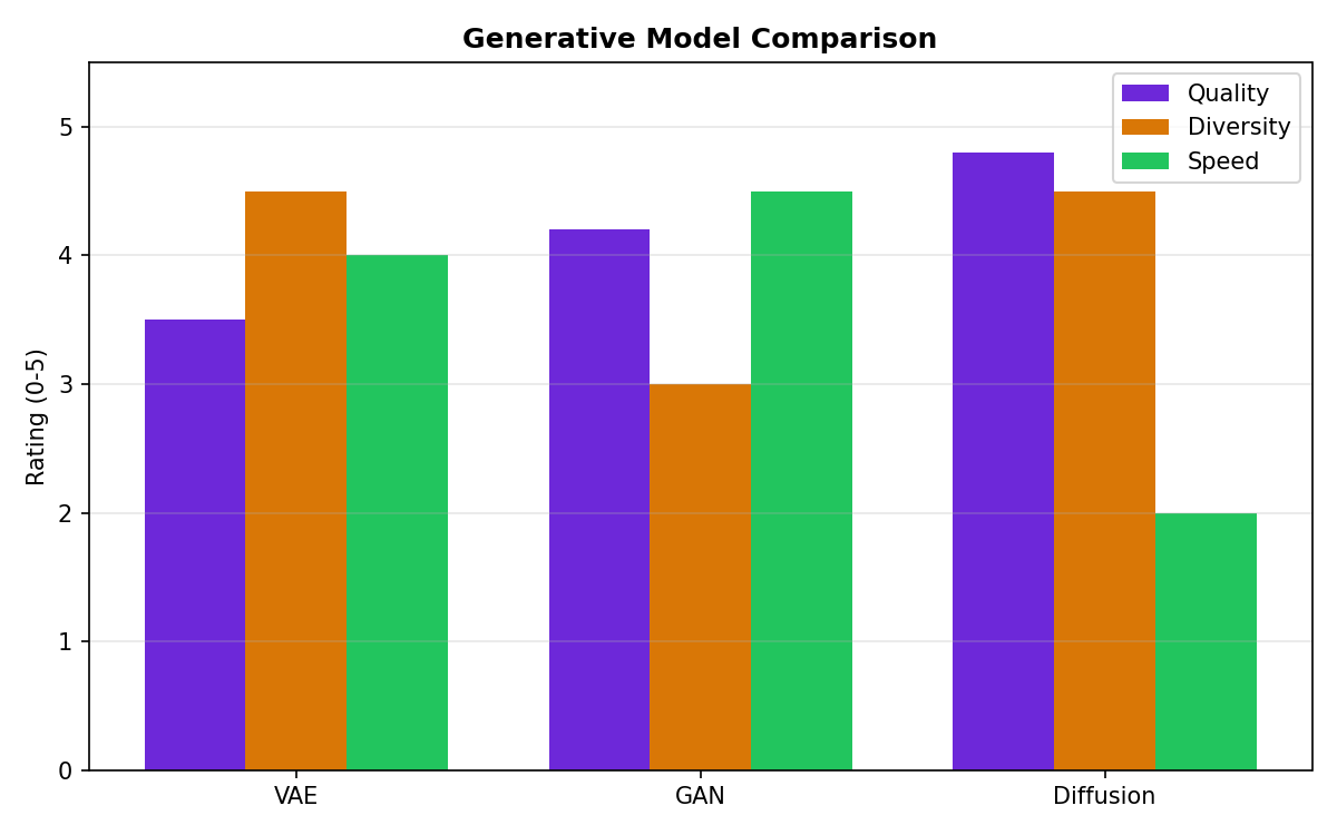
Generative models capture the distribution of real X-rays. Diffusion models currently produce the most realistic samples, followed by GANs. VAE samples are smoother but sometimes less detail-rich.
🎲 VAE for Generation
Recall: VAE learns encoder q(z|x) and decoder p(x|z). The latent space is smooth (regularized by KL divergence). During generation, sample z ~ N(0,1) and decode: x_new = decoder(z).
Why VAE for Generation?
Smooth latent space enables interpolation: z1 and z2 are normal samples; decoder(interpolate(z1, z2)) creates a smooth transition. This is useful for exploring the learned distribution.
VAE Generation Pipeline
🎭 Generative Adversarial Networks (GANs)
A GAN has two networks: generator G and discriminator D. They play a min-max game: G tries to fool D; D tries to distinguish real from fake.
Generator (G)
Maps latent code z → image x_fake. Trains to maximize: log(D(x_fake))—make discriminator believe the fake is real.
Discriminator (D)
Classifies real vs. fake. Trains to maximize: log(D(x_real)) + log(1 - D(x_fake))—correctly identify sources.
GAN Architecture & Training
GAN training progress
Epoch 10 | D Loss: 0.584 | G Loss: 1.263
Epoch 20 | D Loss: 0.512 | G Loss: 1.147
Epoch 30 | D Loss: 0.438 | G Loss: 0.982
...
Epoch 100 | D Loss: 0.324 | G Loss: 0.521
FID Score (lower is better): 42.3 → 18.7
🌊 Diffusion Models (DDPM)
Denoising Diffusion Probabilistic Models (DDPM) iteratively denoise: start with pure noise, gradually denoise to reconstruct an image. This is the SOTA approach as of 2024.
Forward Process
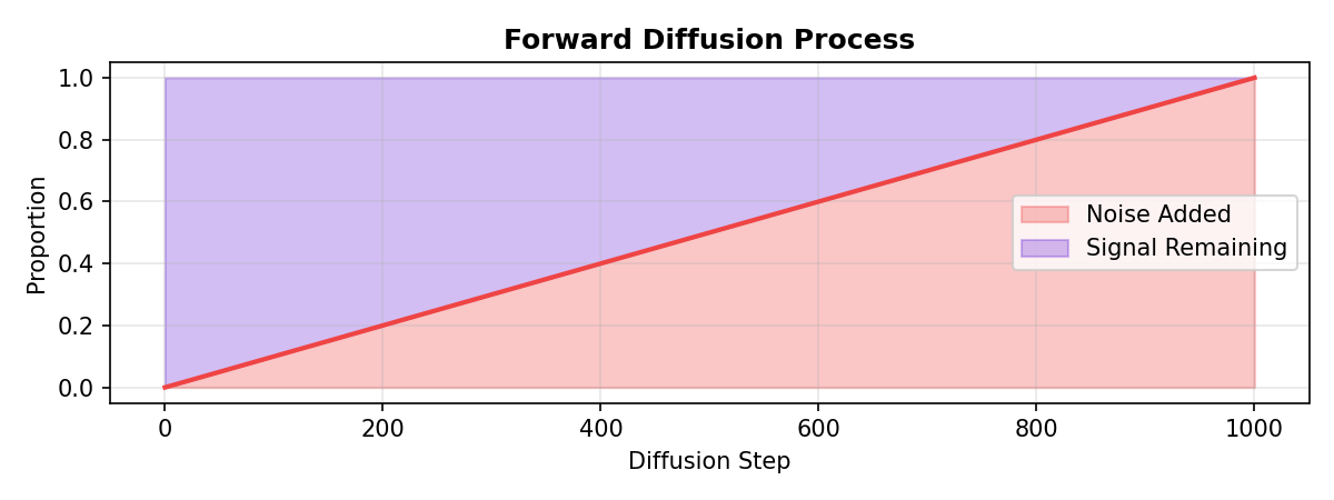
Add Gaussian noise gradually to data: x_0 (real) → x_1 → ... → x_T (pure noise). This is fixed.
Reverse Process
Learn to denoise: x_T (noise) → x_{T-1} → ... → x_0 (image). Parameterize as a neural network that predicts noise at each step.
Diffusion process: forward (add noise) vs. reverse (denoise)
Pros: Sharp, realistic samples. Cons: Training is unstable (mode collapse), hard to debug, limited diversity.
Diffusion
Pros: SOTA quality, stable training, better diversity. Cons: Slow generation (requires many denoise steps), computationally expensive.
🏆 Mini Challenge: Synthetic Data Evaluation
Task: Train a classifier on real X-rays (3.2K). Then retrain on real + 10K synthetic X-rays (VAE, GAN, or Diffusion). Measure AUC on a held-out real test set. Did synthesis help? Which generative model is best?
Hint: Use Frechet Inception Distance (FID) to measure synthetic quality. Combine with downstream task performance (AUC) to choose the best generative model.
💼 Interview Questions
A generative model learns p(x) (data distribution) and can sample new data. A discriminative model learns p(y|x) (decision boundary). Generative: "what are all possible X-rays?" Discriminative: "is this X-ray normal or pneumonia?" Generative is harder but enables data synthesis, interpolation, and understanding of data structure.
A VAE has a smooth latent space (regularized by KL divergence). To generate: (1) sample z ~ N(0, 1), (2) pass through decoder: x_new = decoder(z). The smooth latent space ensures diverse, plausible samples. Arjun generates 10K synthetic X-rays by sampling 10K latent codes.
Generator G and Discriminator D play a min-max game. D wants to maximize: log(D(real)) + log(1 - D(fake))—correctly classify real/fake. G wants to maximize: log(D(fake))—fool D into believing fakes are real. In equilibrium, G learns the data distribution, and D can't distinguish real from fake (D output ~0.5). In practice, training is unstable; gradient issues and mode collapse are common.
Diffusion models have stable, tractable training (just MSE loss for noise prediction). They produce high-quality, diverse samples without mode collapse. The downside: generation requires many denoising steps (~1000), making inference slow. As of 2024, diffusion models (Stable Diffusion, DALL-E 3) have surpassed GANs in quality and adoption.
Mode collapse means G ignores parts of the data distribution to fool D more easily. Fixes: (1) Use spectral normalization in D to stabilize training. (2) Add regularization (gradient penalty, spectral norm). (3) Use Wasserstein distance instead of BCE loss—more stable gradients. (4) Diversify the generator by adding a diversity loss (e.g., minimize similarity between generated samples). (5) Switch to diffusion models—they don't suffer from mode collapse. (6) Use progressive training: start small, gradually increase resolution, giving D/G time to balance.
✓ Quick Quiz
Question 1 / 5
Arjun has only 3.2K X-rays but wants a classifier with 32K training examples. Why is synthesis better than simple augmentation (rotation, flip)?
Question 2 / 5
What is a key advantage of VAE's smooth latent space for generation?
Question 3 / 5
In GAN training, what does mode collapse mean and why is it a problem?
Question 4 / 5
How does diffusion model generation work, conceptually?
Question 5 / 5
You trained a generative model to create synthetic X-rays. How do you verify they are realistic and useful?
Quality + utility; both matter for practical applications
⚠️ Common Mistakes
Evaluating generation with visual inspection alone
Humans can be fooled by realistic-looking samples that don't match the data distribution. Always measure FID (Frechet Inception Distance), IS (Inception Score), or combine quality metrics with downstream task performance (e.g., classifier AUC on real data).
Using synthetic data without domain adaptation
Synthetic X-rays may have subtle artifacts or distribution shift from real scans. When combining real + synthetic for training, monitor performance on a real test set. If AUC drops, your synthetic data may have systematic biases; retrain or improve the generative model.
GAN training instability—not using stabilization tricks
Standard GAN training is unstable. Use: (1) Spectral normalization in D. (2) Gradient penalty (WGAN-GP). (3) Wasserstein distance instead of BCE. (4) Separate learning rates (G: 1e-4, D: 1e-4). (5) Progressive training if possible.
Diffusion model generation too slow
Diffusion requires many denoise steps (~1000). For real-time applications, use DDIM (fewer steps) or distillation. Consider trade-off: fewer steps → faster generation but lower quality.
Not scaling/normalizing images
X-rays are 0-255 or 0-1. Normalize consistently: divide by 255 or use StandardScaler. Diffusion models expect inputs in [-1, 1] or [0, 1]. Mismatched scaling breaks training.
✦ Key Takeaways
Generative models (VAE, GAN, Diffusion) learn p(x) and can sample new data. They enable data augmentation, privacy-preserving sharing, and understanding of data distributions.
VAE: stable training, smooth latent space for interpolation. Diffusion models: SOTA quality, stable training, slower generation.
GAN: sharp samples but training is unstable. Mode collapse limits diversity. Use spectral norm, gradient penalty, or switch to diffusion.
Evaluate generation with FID (quality) and downstream task metrics (utility). Visual inspection alone is insufficient and can be misleading.
Arjun's diffusion-based X-ray synthesis generates 10K diverse, realistic training examples, expanding his dataset 3x and improving diagnostic AUC from 0.88 to 0.94.