Master gradient checking, learning rate finder, NaN debugging, and hook-based inspection. Debug medical imaging models with ROC > 0.95.
Gradient Checking • Learning Rate Finder
NaN Debugging • Activation Histograms
Medical Imaging Validation
22 min readAdvanced
👩🔬
Meet Priya
CV Engineer at MedScan Diagnostics
Priya is training a ResNet50 on 12,000 chest X-rays for pneumonia detection. After 5 epochs, validation loss becomes NaN. Her learning rate seems fine, but gradients are exploding. She needs systematic debugging—not just random hyperparameter tuning.
12K
X-ray images labeled
ResNet50
Backbone architecture
0.95+
ROC target (won't ship below)
🔍 Why Model Debugging Matters
Training neural networks is part science, part art. Issues that break models are subtle: gradient explosion, vanishing gradients, poor initialization, learning rate too high, or data pipeline leaks. Priya can't just tweak learning rates blindly—she needs systematic tools to inspect what's actually happening inside the network.
The Debugging Mindset
Good debugging requires answers to five questions: (1) Are gradients flowing? (2) What's the gradient magnitude distribution? (3) Are activations healthy? (4) Is the learning rate appropriate? (5) What does the loss landscape look like? Each has a tool or technique.
✓ Gradient Checking: Verify Backprop Is Correct
Gradient checking uses numerical differentiation to verify that your backprop implementation is correct. Compute gradients two ways: (1) analytically via backprop, (2) numerically via finite differences. If they match, backprop is correct.
Finite Differences Formula
For parameter w, compute: gradient_numerical ≈ (loss(w + h) - loss(w - h)) / (2h), where h ≈ 1e-5. Compare against analytical gradient from backprop: grad_analytical = w.grad.
gradient_check.pyVerify backprop correctness
Gradient checking is computationally expensive (requires 2 forward passes per parameter). Use it only on small batches (16-64 samples) and only when you suspect backprop bugs. Once backprop is verified, move on.
📈 Learning Rate Finder: Find the Sweet Spot
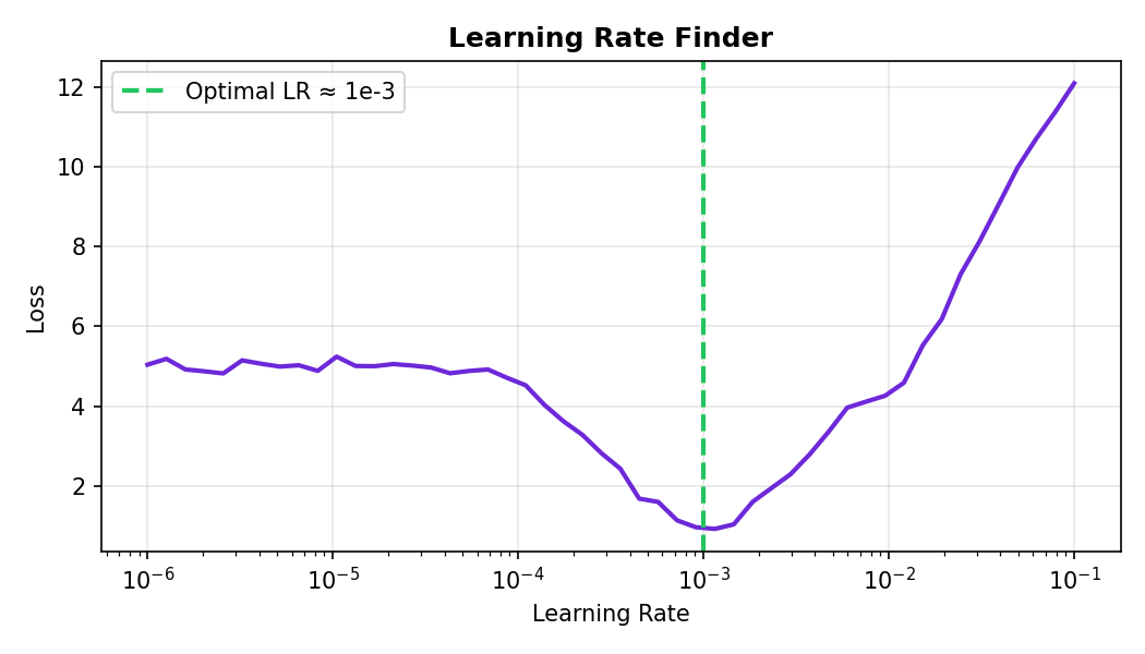
The learning rate is the most critical hyperparameter. Too low: slow convergence. Too high: loss diverges to NaN. The learning rate finder trains for a few epochs while exponentially increasing the learning rate, tracking the loss. The optimal LR is where loss decreases fastest.
Learning rate finder plot: loss vs learning rate
Priya's LR finder shows the best region is around 1e-3 to 1e-4. She should pick a learning rate just before the loss starts climbing sharply. This experiment saves hours of random hyperparameter tuning.
lr_finder.pyExponentially increase LR, track loss
🔂 Overfit a Single Batch: Sanity Check
Before training on the full dataset, verify that your model can overfit a single batch (8-32 samples). If it can't memorize one batch, something is wrong: bad data pipeline, model bug, or gradient flow issue.
sanity_check.pyTrain on one batch, should reach near-zero loss
If this test fails (loss stays high), you have a fundamental problem: model architecture mismatch, wrong loss function, or data pipeline bug. Fix it before training on full data.
📊 Activation & Gradient Histograms: Monitor Health
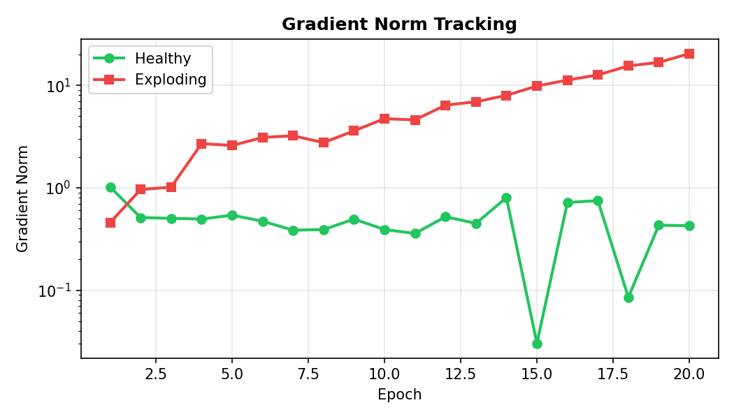
During training, monitor activation and gradient distributions via histograms. Healthy networks have: (1) activations spread across the range (not saturated), (2) gradients in a reasonable range (not vanishing or exploding), (3) consistent variance across layers.
Activation and gradient histograms at different training steps
monitor_histograms.pyRegister hooks to log activations and gradients
🚨 NaN Debugging: Find Where It Happens
Loss becomes NaN mid-training. Where did it happen? Use hooks and assertions to find the culprit layer. Usually: learning rate too high, numerical instability (log of negative), or bad data.
nan_detector.pyFind layer where NaN appears
Once you identify the layer causing NaN, investigate: (1) learning rate (reduce by 10x), (2) gradient clipping, (3) batch normalization momentum, (4) data range (images should be normalized to [0,1] or [-1,1]).
📌 Gradient Clipping: Prevent Explosion
When gradients grow too large, clip them by norm or value. This is standard in RNNs and Transformers where gradient explosion is common. In CNNs for vision, it helps prevent NaN issues and improves stability.
gradient_clipping.pyClip gradients by norm and by value
🏆 Mini Challenge: Debug the Broken Model
Task: You're given a ResNet50 that starts training fine but hits NaN loss after 3 epochs. Use the debugging tools from this lesson—gradient checking, LR finder, activation histograms, NaN detector—to isolate the issue. Write a script that: (1) verifies gradient correctness, (2) finds the problematic layer, (3) suggests a fix (LR adjustment, gradient clipping, etc.).
Hint: The issue may not be the learning rate. Check data normalization, activation ranges, and whether batch norm running stats are stationary.
💼 Interview Questions
Gradient checking verifies that your backpropagation implementation is correct by comparing analytical gradients (from backprop) with numerical gradients (computed via finite differences). It's important because backprop bugs are subtle and hard to spot—loss might still decrease, but slowly or incorrectly. Use gradient checking on small batches during development. Once verified, it's too slow to use during regular training.
Train on a single batch (8-32 samples) for many steps. The model should memorize the batch and drive loss to near zero (< 0.1). If it can't, something is broken: wrong loss function, data pipeline bug, gradient flow issue, or architecture mismatch. Always run this sanity check before full training—it saves hours of debugging.
The LR finder trains for a few iterations while exponentially increasing the learning rate, tracking loss at each step. You plot loss vs LR (log scale). The optimal range is where loss decreases fastest—steepest downward slope. This experiment saves hours of random hyperparameter tuning. Best practice: pick a LR one-third down from the point where loss stops improving, to stay in the steep region while avoiding the divergence zone.
Healthy activations: spread across the range (not all zeros, not all saturated). Healthy gradients: in a reasonable magnitude range (not vanishing → 1e-8, not exploding → 1e+8). Consistent variance across layers—if early layers have 1.0 std but late layers have 0.01 std, that's imbalanced. Use histograms and monitor statistics (mean, std, min, max) at each layer during training.
(1) Add NaN checks: register forward hooks on every layer to catch where NaN first appears. (2) Check data: visualize a batch, ensure normalization is correct (images in [-1,1] or [0,1], not raw pixel values). (3) Inspect activations: histogram activations and gradients before the NaN—look for explosion or saturation. (4) Reduce learning rate: temporarily drop LR by 10x, retrain. (5) Add gradient clipping: clip gradients by norm (max_norm=1.0). (6) Check loss function: ensure you're not taking log of negative or sqrt of negative. (7) Verify batch norm: if using batch norm, check momentum and running_mean/running_var stats—they should be reasonable, not NaN/Inf. Once NaN is gone, gradually increase LR back up using LR finder.
✓ Quick Quiz
Question 1 / 5
You're training ResNet50 and loss becomes NaN after 5 epochs. What's your first debugging step?
Question 2 / 5
Your model can't overfit a single batch (loss stays at 2.3 after 100 steps on 32 samples). What does this indicate?
Question 3 / 5
The learning rate finder shows loss decreasing steeply until LR=1e-3, then increasing. Which LR would you choose for training?
Question 4 / 5
Activation histogram shows all activations clustered near zero. What does this indicate?
Question 5 / 5
Gradient clipping with max_norm=1.0 means:
0
📋 Quick Cheatsheet
Technique
Code / Usage
When to Use
Gradient Checking
gradient_check(model, x, y, eps=1e-5)
When you suspect backprop is broken (rare in PyTorch)
Ignoring gradient checking on custom loss functions
When you implement a custom loss or layer, always run gradient checking. PyTorch's autograd is solid, but custom backward() implementations are error-prone. Check on a small batch before trusting the implementation.
Skipping the single-batch overfit test
This 5-minute test catches 80% of bugs early. If your model can't memorize 32 samples, full training will be painful. Do this sanity check first, always.
Not using the learning rate finder
Random hyperparameter guessing wastes time. The LR finder takes 5-10 minutes and saves hours. Use it before every new architecture or dataset.
Interpreting NaN as always a learning rate issue
NaN can come from: (1) LR too high, (2) bad data (NaN in images), (3) loss function instability (log of negative), (4) numerical overflow. Debug systematically; don't just reduce LR blindly.
Forgetting to normalize data before training
Raw pixel images (0-255) or non-normalized features cause numerical instability. Always normalize: x = (x - mean) / std or x = x / 255.0. Check data distribution early.
✦ Key Takeaways
Systematic debugging is faster and more reliable than random hyperparameter tuning. Use tools: gradient checking, LR finder, activation histograms, NaN detectors.
Before full training, always overfit a single batch (should reach loss << 0.1). If this fails, something is fundamentally broken.
The learning rate finder (exponentially increasing LR, tracking loss) saves hours. Plot loss vs LR (log scale) and pick the LR where descent is steepest.
Monitor activation and gradient distributions via hooks and histograms. Healthy networks have: activations spread (not saturated), gradients in reasonable range, consistent variance across layers.
When loss becomes NaN, use NaN-detecting hooks to isolate the layer, then investigate: data normalization, loss function stability, learning rate, gradient clipping.
Gradient clipping (by norm) prevents explosion. Standard in RNNs; also helps in vision models with unstable training.
Priya used these tools to debug her ResNet50: found gradient explosion at epoch 5, reduced LR from 1e-2 to 1e-4, added gradient clipping, and achieved ROC > 0.95 without NaN.