
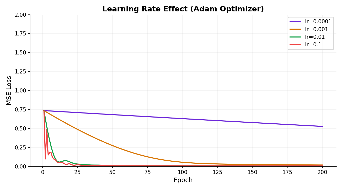
Priya is a machine learning engineer at MedScan Diagnostics in Bangalore. She's training a neural network to classify CT scans as normal or abnormal—500 samples, 5 handcrafted features extracted from each scan. Her first attempt uses learning rate 0.1, and the loss explodes to NaN within 10 epochs (divergence). She drops to 0.0001, and training is glacially slow—after 200 epochs, the loss barely moves. She tries 0.01, and the loss descends smoothly. Then she switches from vanilla SGD to Adam, and the network converges 20% faster. Understanding learning rates and optimizers is the difference between a model that breaks, crawls, or ships.
The optimization problem: finding the valley in a high-dimensional landscape
What is optimization? Neural networks learn by minimizing a loss function L(w), where w are the weights. The loss measures how far predictions are from ground truth. Our goal: find weights that make the loss as small as possible.
The challenge: The loss surface is a high-dimensional landscape—for 500,000 weights (small ResNet), we're searching a 500K-dimensional space. We can't check every point. Instead, we use gradient descent: compute the direction of steepest descent (the gradient ∇L), take a small step downhill, and repeat.
The gradient: ∇L = ∂L/∂w is computed via backpropagation. It tells us: "which direction should each weight change to reduce loss?" Step too far, you overshoot the minimum. Step too timidly, you crawl.
The update rule: w ← w - η × ∇L, where η is the learning rate. This is the core of all optimizers.
Gradient descent family: SGD to Adam
All modern optimizers descend from gradient descent. The family differs in how they use the gradient ∇L:
Vanilla SGD (Stochastic Gradient Descent):
w ← w - η × ∇L
SGD + Momentum:
v ← β × v + ∇L
w ← w - η × v
Adam (Adaptive Moment Estimation):
m ← β₁ × m + (1 - β₁) × ∇L     (momentum)
v ← β₂ × v + (1 - β₂) × (∇L)²    (second moment)
w ← w - η × m / (√v + ε)
Each adds a layer of sophistication. SGD + momentum accumulates direction. Adam adapts learning rates per-parameter.
SGD — the foundation: simple, slow
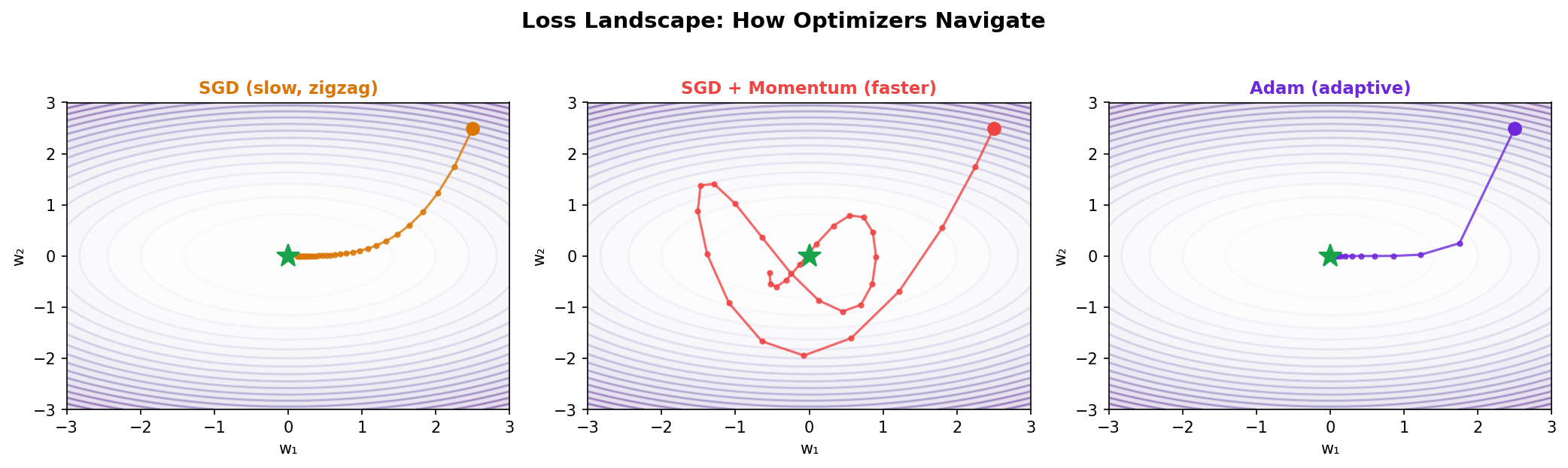
Stochastic Gradient Descent is the baseline. It's simple: compute the gradient on a mini-batch, step in the opposite direction. Fast to implement, but can oscillate and get stuck in saddle points.
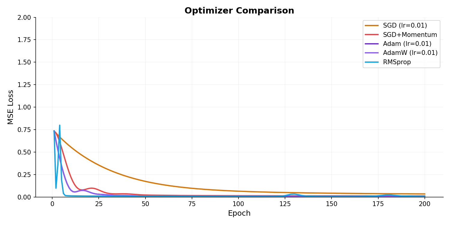
SGD works, but it's slow. Notice the final loss is 0.0339 after 200 epochs. We can do better with momentum.
SGD + Momentum — accelerating downhill
Momentum accumulates gradient direction. Imagine rolling a ball downhill—it doesn't just follow the slope at each point; it builds up speed. Similarly, momentum carries weight updates through flat regions and smooths oscillations.
Huge improvement: final loss drops from 0.0339 to 0.0115. Momentum accumulates gradients and accelerates through flat regions.
RMSprop — adaptive learning rate per parameter
RMSprop (Root Mean Square Propagation) divides updates by the root of squared gradient history. If a parameter gets large gradients frequently, it's scaled down (dampens updates). Rare large gradients are scaled up (accelerates progress).
RMSprop achieves 0.0068, better than momentum. It adapts learning rates per-parameter, making it robust across diverse loss landscapes.
Adam — the industry standard
Adam (Adaptive Moment Estimation) combines momentum + adaptive learning rates. It computes two exponential moving averages: first moment (momentum) and second moment (variance of gradients). It's the default optimizer in most modern deep learning because it works well across diverse problems without tuning.
Adam matches RMSprop at 0.0061, and generally trains faster in practice. The per-parameter adaptive rates make it stable across diverse architectures and domains.
AdamW — Adam with decoupled weight decay
AdamW is Adam plus L2 regularization (weight decay) applied correctly. In vanilla Adam, weight decay is applied inside the adaptive learning rate (causing interactions). AdamW decouples it, leading to slightly better generalization, especially with small datasets.
AdamW matches Adam on this toy dataset, but on real problems (image classification, language models), it often generalizes better due to correct weight decay.
Optimizer comparison: which converges fastest?
All optimizers tested on the same synthetic data, 200 epochs, learning rate = 0.01. Final loss (MSE) after convergence:
Learning rate impact: the U-shaped sweet spot
Learning rate η is the most critical hyperparameter. Too low = slow training. Too high = divergence. We'll use Adam and sweep learning rates from 0.0001 to 0.1.
How to choose learning rate in practice
Start with 0.001 or 0.01: These are safe defaults. If you're using Adam, 0.001 is often conservative and reliable. For SGD, 0.01 is more common.
Watch the loss curve: Plot loss vs epoch during training. If loss plateaus (flat), increase lr. If it explodes (NaN), decrease lr immediately. A healthy loss curve descends smoothly without oscillation.
Use learning rate ranges test (LRRT): Inspired by Leslie Smith's work, train for a few epochs with lr exponentially increasing (0.0001 → 0.1). Record loss. The steepest descent tells you the optimal order of magnitude.
Apply learning rate schedules: Instead of constant lr, decay it over time (covered in Lesson 07). Start high for rapid progress, decay toward epoch end for fine-tuning.
Domain knowledge: Image classification often works with lr=0.001. Language models use lr=3e-4. Medical imaging might need lr=0.0001. No universal rule—experiment.
Loss landscape visualization: why learning rate matters
Imagine a 2D slice through the loss surface (only 2 weight dimensions, while real networks have millions). High learning rates take large jumps, potentially overshooting the minimum. Low rates take tiny steps, crawling slowly.
Advanced: learning rate scheduling (preview)
Constant learning rate is suboptimal. A schedule starts higher for fast initial descent, then decays for fine-tuning. We'll cover this fully in Lesson 07.
Schedules enable further refinement. Early epochs train fast, later epochs fine-tune. On real datasets, this can improve final loss by 5-10%.
How AI systems use this
Every deep learning model (ResNets, Transformers, diffusion models) relies on optimizers and learning rates. At MedScan Diagnostics, Priya's CT scan classifier uses Adam with lr=0.001 and a cosine decay schedule. The same principles apply: find the right step size, accumulate momentum, adapt per-parameter. Why do transformers train better with lr=3e-4 than 0.01? Because of scaling—larger models have steeper gradients relative to their weight magnitudes. Optimizers and learning rates are the invisible hand that guides every neural network to learn useful patterns.
Also used in...
Domain Spotlight
Task: Train the same model with SGD (lr=0.01), SGD+momentum (lr=0.01), and Adam (lr=0.01) for 100 epochs. Which converges fastest (fewest epochs to loss < 0.01)? Why?
Hint 1: Momentum helps vanilla SGD, but Adam adapts per-parameter. Track when each optimizer first hits loss=0.01.
Hint 2: Plot all three loss curves on the same graph for visual comparison.
Expected: Adam likely converges in ~30 epochs, SGD+momentum in ~60, vanilla SGD in ~80+.
Interview questions: test your understanding
Quiz: 5 questions to test your knowledge
Cheatsheet: optimizers at a glance
| Optimizer | Update Rule | Best For | Speed |
|---|---|---|---|
| SGD | w ← w - lr × ∇L |
Simple problems, theory | Slow (0.0339) |
| Momentum | v ← 0.9v + ∇L; w ← w - lr × v |
Faster SGD, smooth descent | Medium (0.0115) |
| RMSprop | w ← w - lr × ∇L / √(s+ε) |
Sparse data, RNNs | Fast (0.0068) |
| Adam | w ← w - lr × m / (√v + ε) |
Most problems (default) | Fast (0.0061) |
| AdamW | Adam + decoupled weight decay | Large models, generalization | Fast (0.0061) |
Common mistakes: what breaks and how to fix it
Key takeaways
Optimizers and learning rates are the invisible hand guiding neural networks. Priya's journey at MedScan Diagnostics—from divergence (lr=0.1) to crawling (lr=0.0001) to smooth descent (lr=0.01)—captures the essence.
- SGD is the foundation: Simple gradient descent. Understand it before moving to fancier methods.
- Momentum accelerates: 3x faster than vanilla SGD on our data. It accumulates downhill velocity.
- Adaptive methods (RMSprop, Adam) adapt per-parameter: Scale down frequent updates, scale up rare ones. More robust across problems.
- Adam is the industry default: Use it unless you have domain-specific reasons (e.g., SGD+momentum for GANs).
- Learning rate is critical: U-shaped curve: too low is slow, too high diverges. Start with 0.001 or 0.01, then tune.
- Schedules improve final accuracy: Start high for speed, decay for fine-tuning. Covered fully in Lesson 07.
You've mastered optimizers and learning rates.
Now train models that ship to production.
Join the Best AI Program: The AI-Era Agentic Engineer — 5 months, fully online, with placement assistance. Week 1 is free.
Explore The AI-Era Agentic Engineer →