
Arjun is an ML engineer at MedScan Diagnostics in Bangalore. His team built a classification model to predict whether insurance charges exceed $15,000 (which correlates with medical risk). The model works, but he can't explain why. He traces the issue back to the simplest building block: a single perceptron neuron. By implementing it from scratch in NumPy, he understands the learning algorithm. Then he rebuilds it in PyTorch to see how frameworks automate the math—and why understanding the foundations matters before scaling to deep networks.
The perceptron isn't magic. It's a supervised learner that updates weights when it makes mistakes. Every neuron in every modern deep network follows this same principle, just in parallel and with non-linear activations. This lesson is the DNA of deep learning.
Anatomy of a perceptron: the simplest neuron
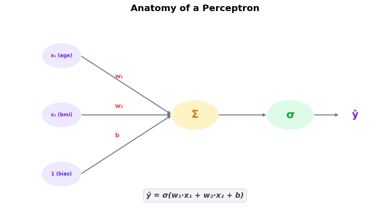
A perceptron has four core parts: inputs, weights, bias, and an activation function. Here's how they connect:
Four-step forward pass
1. Inputs: Six features (age, BMI, smoker status, region, children, sex) feed in as x₁, x₂, ..., x₆.
2. Weighted sum: Each input is multiplied by a weight (w₁, w₂, ..., w₆) and summed with bias b. The result is z = w₁x₁ + w₂x₂ + ... + w₆x₆ + b.
3. Activation: The linear sum z is passed through an activation function. Originally, the perceptron used a step function: output 1 if z ≥ 0, else 0. Modern versions use sigmoid: σ(z) = 1/(1+e^-z), which is differentiable and enables backpropagation.
4. Prediction: The activated output is the neuron's prediction. If sigmoid output ≥ 0.5, classify as 1 (high charges); else 0 (low charges).
The learning rule: how the perceptron learns
The perceptron's magic is the learning algorithm. When it mispredicts, it adjusts its weights to correct the error.
The perceptron learning rule
For each training sample, compute:
z = Σ(w_i × x_i) + b— linear combinationy_pred = 1 if z ≥ 0 else 0— binary predictionerror = y_true - y_pred— 0 if correct, ±1 if wrongw ← w + η × error × x— update weights by learning rate η and error scaled by the inputb ← b + η × error— update bias the same way
Intuition: If the perceptron predicts 0 but should predict 1 (error = 1), it increases the weights in the direction of the input. This nudges the next prediction closer to 1. If it predicts 1 but should predict 0 (error = -1), it decreases the weights, pushing the prediction toward 0.
Convergence: If the data is linearly separable, this algorithm converges in finite epochs. If not (like the insurance data with 89.8% accuracy), it stops oscillating after enough iterations and settles into the best linear boundary.
Step 1: NumPy Perceptron from scratch
Build the perceptron by hand. This is educational—you'll see every line of the learning algorithm.
Decision boundary: where the perceptron splits the data
The weights define a linear decision boundary in the 6D input space. In 2D projections, we can visualize how well the perceptron separates high and low charges.
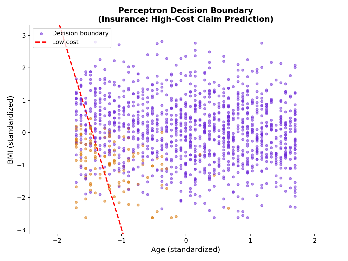
The perceptron found a linear boundary, but it doesn't perfectly separate the classes (that's why accuracy is 89.8%, not 100%). Some high-charge patients fall on the "low" side of the boundary, and vice versa. This is the limitation of linear classifiers—they can't learn non-linear patterns. That's why we stack multiple perceptrons (Multi-Layer Perceptron) in the next lesson.
From step function to sigmoid: enabling backpropagation
The original perceptron used a step function (0 or 1), which is non-differentiable. Modern neural networks use sigmoid, which is smooth and has a gradient everywhere.
Why sigmoid matters
Step function: y = 1 if z ≥ 0 else 0. Sharp cutoff, no gradient. Gradient is 0 everywhere except the discontinuity. Backpropagation can't flow through it.
Sigmoid: σ(z) = 1 / (1 + e^-z). Smooth S-curve from 0 to 1. Gradient is σ(z) × (1 - σ(z)), which is non-zero everywhere. Enables backpropagation to compute gradients all the way to input.
Trade-off: Sigmoid is more gradual, so the perceptron doesn't make hard 0/1 decisions. Instead, it outputs a probability: the higher the sigmoid output, the more confident it is that the sample is class 1. We threshold at 0.5 for the final prediction.
Your PyTorch code below will use sigmoid + BCE loss, not the Hebbian rule. BCE (Binary Cross-Entropy) is the standard loss for probabilistic classifiers. It penalizes wrong predictions more when the model is confident, pushing the model to learn better boundaries.
Step 2: PyTorch Perceptron—same neuron, automated math
PyTorch replaces manual weight updates with automatic differentiation. You define the architecture; PyTorch handles gradients and optimization.
Training progress: loss over time
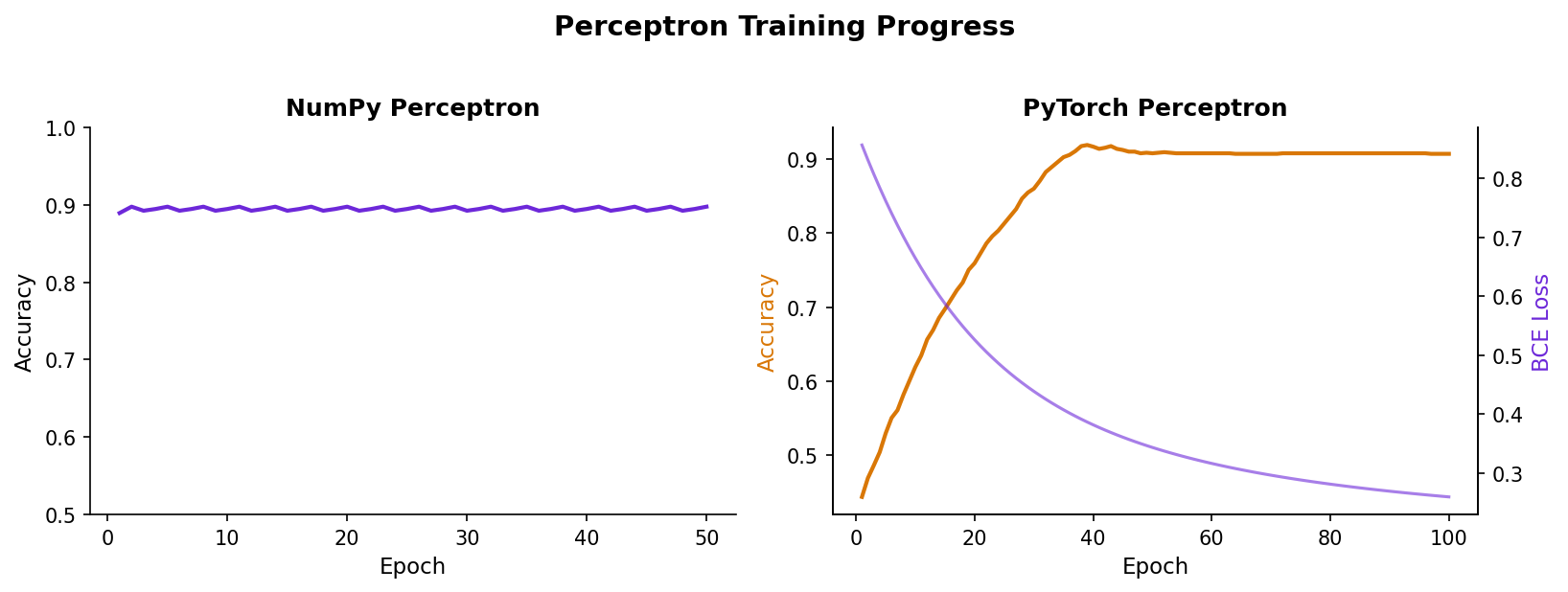
As the perceptron trains, the loss decreases. The steeper drops early on show the model learning quickly; the plateau later shows it's found a local optimum.
Why the perceptron matters: the DNA of deep learning
The perceptron is not just a historical footnote
A neural network with 10 hidden layers and 1000 neurons per layer contains 10,000 perceptron-like units, all learning simultaneously via backpropagation. Each one updates its weights based on the error signal flowing backward through the network. The principles are identical:
- Linear combination: z = w^T x + b (same in every neuron, every layer)
- Activation: Modern networks use ReLU, sigmoid, tanh—all smooth functions with non-zero gradients
- Learning: Gradient descent updates w ← w - α ∇L(w) (same algorithm, scaled to millions of parameters)
The single perceptron is the atom. Deep neural networks are atoms organized into molecules. Understanding the atom is prerequisite to understanding the molecule.
Limitations: why one neuron isn't enough
The perceptron can only solve linearly separable problems. It can draw a single straight line (in 2D) or hyperplane (in higher dimensions) to split the data. But many real problems require non-linear boundaries.
- XOR problem: Can a perceptron learn XOR? No. XOR requires two lines to separate the true cases from false—a single hyperplane can't do it.
- Insurance charges: Our perceptron achieved 89.8%, but 10% of samples still misclassify. Many combinations of age, BMI, smoker status, and region don't fit a simple linear pattern. Charges might jump non-linearly with age for smokers but not non-smokers.
- Image recognition: A perceptron on raw pixel values can't recognize a cat. The relationship between pixel patterns and "cat" is highly non-linear.
The solution: stack multiple perceptrons with non-linear activations (ReLU). The hidden layers learn non-linear features that feed into the output layer. This is a Multi-Layer Perceptron (MLP), and it solves XOR and much harder problems. That's the subject of the next lesson.
How AI systems use this
Every deep learning model—language transformers, image classifiers, recommendation systems—is built from perceptron-like units. The transformer in ChatGPT has millions of "neurons" (actually called attention heads and feed-forward layers), each one following the perceptron principle: linear transformation + non-linear activation + gradient-based learning. The perceptron is the conceptual foundation of all modern AI.
Also used in...
Domain Spotlight
Task: Train the NumPy perceptron three times with learning rates 0.001, 0.01, and 0.1. Plot the accuracy for each. Which learning rate converges fastest? Which overshoots and oscillates?
Hint 1: Loop over learning rates: for lr in [0.001, 0.01, 0.1]:
Hint 2: For each lr, train the perceptron and record test accuracy at epochs 10, 20, 30, ..., 50.
Hint 3: Plot with matplotlib: plt.plot(epochs, accuracies, label=f'lr={lr}')
Expected: lr=0.001 converges slowly (low accuracy until epoch 50). lr=0.01 is balanced (smooth convergence). lr=0.1 might overshoot early then stabilize.
Interview questions: test your understanding
Quiz: 5 questions to test your knowledge
Cheatsheet: perceptron components at a glance
| Component | Equation | Role |
|---|---|---|
| Linear combination | z = Σ(w_i × x_i) + b |
Compute neuron input as weighted sum |
| Sigmoid activation | σ(z) = 1 / (1 + e^-z) |
Squash output to (0, 1) probability |
| Prediction | y_pred = 1 if σ(z) ≥ 0.5 else 0 |
Binary classification output |
| Error | error = y_true - y_pred |
Measure misprediction signal |
| Weight update | w ← w + η × error × x |
Adjust weights by learning rate and error |
| BCE Loss | -[y log(ŷ) + (1-y) log(1-ŷ)] |
Continuous loss for probabilistic output |
Common mistakes: what breaks and how to fix it
torch.sigmoid(z) or torch.relu(z).StandardScaler() scales all features to mean 0, std 1. Learning becomes stable and fast.You've built a neuron from scratch.
Now scale it to production neural networks.
Join the Best AI Program: The AI-Era Agentic Engineer — 5 months, fully online, with placement assistance. Week 1 is free.
Explore The AI-Era Agentic Engineer →