
Thomas works as a financial data analyst at SouthBank India in Kochi. Every Monday morning, he manually copies customer transaction data from the PostgreSQL warehouse into an Excel file. He writes SQL queries in the database GUI, pastes the results into Excel, then transforms them in pandas. It takes 40 minutes and is error-prone.
Last week, he wrote a 3-line Python script that queries PostgreSQL directly into a DataFrame. No copying. No pasting. No waiting. Every query runs in seconds, fresh data every time.
The transformation: from SQL query to analysable DataFrame
Below, the same query appears twice: left as SQL in the database, right as a styled DataFrame after pd.read_sql() loads it. Notice how column names are preserved and amounts are properly formatted.
pd.read_sql()
| customer_id | total_spend |
|---|---|
| 1027 | ₹8,45,200 |
| 1003 | ₹7,92,500 |
| 1041 | ₹7,65,800 |
| 1015 | ₹7,23,400 |
| 1009 | ₹6,98,900 |
| 1022 | ₹6,54,300 |
| 1035 | ₹6,21,100 |
| 1008 | ₹5,89,700 |
| 1019 | ₹5,34,200 |
| 1012 | ₹4,97,600 |
Three ways to talk to a database
You can connect to SQL databases from Python in different ways. Each has trade-offs. Here are the most common:
| Method | Best for | Trade-off |
|---|---|---|
psycopg2 (PostgreSQL) or mysql.connector |
Fine-grained control, low-level database ops | Verbose; you manage connections, cursors, result iteration yourself |
SQLAlchemy |
Production code, ORM-style queries, database-agnostic applications | Steep learning curve; overkill for one-off scripts |
pd.read_sql() + SQLAlchemy engine |
Data analysis workflows (THIS COURSE) | Best of both worlds: simple, Pythonic, works with all major databases |
For this lesson and most analysis work, we use pd.read_sql() + SQLAlchemy. Write your SQL query, pass an engine, get a DataFrame back in one line.
The 3-line setup: connect, query, analyse
Here's the minimal code to load SouthBank transaction data from a PostgreSQL database into a DataFrame:
| customer_id | total_spend |
|---|---|
| 1027 | 8452.00 |
| 1003 | 7925.00 |
| 1041 | 7658.00 |
| 1015 | 7234.00 |
| 1009 | 6989.00 |
Four patterns: filter, aggregate, join, window function
Most SQL-to-pandas workflows follow one of these patterns. Learn these, and you can handle 80% of real-world queries.
Pattern A: Filter + Aggregate (top spenders per month)
Find the top 10 customers by total spend across all of 2026. Simple filtering and aggregation—the bread and butter of analysis.
| name | segment | txn_count | total_spend |
|---|---|---|---|
| Priya | premium | 18 | ₹8,45,200 |
| Vikram | standard | 16 | ₹7,92,500 |
| Anjali | premium | 15 | ₹7,65,800 |
| Rohan | basic | 14 | ₹7,23,400 |
| Deepika | standard | 17 | ₹6,98,900 |
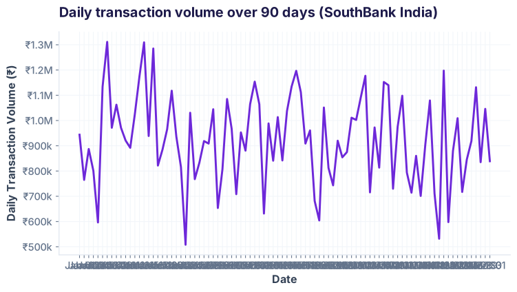
Pattern B: Time-series with GROUP BY DATE (daily volume over 90 days)
Detect trends, seasonality, anomalies. Group by date, count or sum, plot. This unlocks time-based analysis that Excel pivot tables can't match.
Pattern C: JOIN (customer names + transaction details)
Combine customers and transactions tables to get names, cities, segments, and transaction amounts in one result. This mirrors real-world schemas.
| customer_id | name | city | segment | txn_date | amount | category |
|---|---|---|---|---|---|---|
| 1027 | Priya | Mumbai | premium | 2026-03-28 | ₹75,000 | utilities |
| 1041 | Anjali | Bangalore | premium | 2026-03-27 | ₹72,500 | fuel |
| 1027 | Priya | Mumbai | premium | 2026-03-26 | ₹68,900 | groceries |
| 1015 | Aditya | Hyderabad | premium | 2026-03-25 | ₹65,200 | entertainment |
| 1022 | Meera | Chennai | premium | 2026-03-24 | ₹61,800 | healthcare |
Pattern D: Window functions (rank top 3 per branch)
Find top spenders per branch using RANK() OVER PARTITION BY. Window functions are SQL's superpower for comparative rankings.
| name | branch | branch_spend | rank_in_branch |
|---|---|---|---|
| Vikram | Bangalore | ₹2,34,500 | 1 |
| Pooja | Bangalore | ₹2,12,300 | 2 |
| Sanjay | Bangalore | ₹1,98,700 | 3 |
| Priya | Chennai | ₹2,45,800 | 1 |
| Rashmi | Chennai | ₹2,18,900 | 2 |
| Deepika | Chennai | ₹2,05,400 | 3 |
Security: parameters, not string concatenation
Never build SQL queries by pasting user input into strings. SQL injection is a real attack vector. Always use parameterized queries.
user_id = input("Enter customer ID: ")
query = f"SELECT * FROM customers WHERE customer_id = {user_id}"
# If user enters: 1 OR 1=1
# Query becomes: SELECT * FROM customers WHERE customer_id = 1 OR 1=1
# Result: attacker sees ALL customer data!
user_id = input("Enter customer ID: ")
query = "SELECT * FROM customers WHERE customer_id = %(id)s"
df = pd.read_sql(query, engine, params={'id': user_id})
# The database driver escapes the input
# Query is safe, even if user enters malicious input
%(name)s placeholders and pass params as a dictionary. The database driver handles escaping. Even if a user enters SQL commands, they're treated as literal values, not code.
When to filter in SQL vs pandas
You can filter and aggregate in SQL, or load raw data and work in pandas. Which is faster? Use this guide:
| Operation | Do in SQL | Do in pandas | Why |
|---|---|---|---|
| Filter rows | WHERE date > 2026-01-01 | df[df['date'] > '2026-01-01'] | SQL filters at the source; pandas loads everything then filters (slower on huge data) |
| Aggregate (sum, count, avg) | GROUP BY, SUM() | df.groupby().sum() | SQL aggregates in the database engine (optimized); pandas does it in memory |
| JOIN tables | JOIN ... ON ... | df.merge() | SQL joins are database-optimized; pandas merge is slower on large tables |
| Reshape / pivot | CASE WHEN (verbose) | df.pivot(), df.melt() | Pandas pivot syntax is cleaner; SQL PIVOT is database-specific |
| Plot / visualize | Not applicable | matplotlib, seaborn | Python plotting is the entire point of pandas |
| Machine learning features | Not applicable | df['new_col'] = ... | Python is where ML libraries live (sklearn, xgboost) |
Rule of thumb: Filter and aggregate in SQL. Shape, plot, and model in pandas. This splits work where each tool excels.
SQL + pandas cheatsheet
| Task | Code |
|---|---|
| Connect to SQLite | engine = create_engine('sqlite:///southbank.db') |
| Connect to PostgreSQL | engine = create_engine('postgresql://user:pwd@localhost/dbname') |
| Connect to MySQL | engine = create_engine('mysql+pymysql://user:pwd@localhost/dbname') |
| Load entire table | df = pd.read_sql_table('transactions', engine) |
| Run SQL query | df = pd.read_sql('SELECT * FROM transactions', engine) |
| Query with parameters | pd.read_sql(query, engine, params={'id': user_id}) |
| Filter by date range | WHERE txn_date BETWEEN '2026-01-01' AND '2026-03-31' |
| Aggregate by group | GROUP BY customer_id, branch |
| LIMIT results | LIMIT 100 |
| Inner JOIN | JOIN customers c ON t.customer_id = c.customer_id |
| Rank within group | RANK() OVER (PARTITION BY branch ORDER BY amount DESC) |
| Convert result to CSV | df.to_csv('output.csv', index=False) |
Task: Using the southbank.db sample database, write a query that finds the 5 customers with the highest total spend in the last 90 days (Jan 1 – Mar 31, 2026). Your result should show: customer_id, customer name, total spend, and number of transactions.
Bonus: Which customer has the highest average transaction amount?
You'll need:
- JOIN transactions to customers
- WHERE to filter the date range
- GROUP BY customer
- SUM(amount) and COUNT(*) for aggregates
- AVG(amount) for the bonus
- ORDER BY total_spend DESC
- LIMIT 5
5 common pitfalls (and how to avoid them)
conn.close(). With create_engine(), pandas handles cleanup. But if you open raw connections, they stay open and drain resources.SELECT * will crash your laptop. Always start with LIMIT 1000 to preview. Then add WHERE filters to narrow the result set before loading all data.df['time'].dt.tz_convert('Asia/Kolkata')."CustomerID" (PostgreSQL) vs `CustomerID` (MySQL).LIMIT 100 during development, remove it only after testing on sample data.Interview questions
Quick quiz
Where else you'll use this
Domain applications
How AI uses SQL + pandas
Large language models like ChatGPT are trained to generate SQL queries from plain-English prompts. You say "find customers who spent more than ₹100k in March", and the AI generates the WHERE clause. But the AI can't validate whether the query is correct until a human reviews it and runs it against real data.
This is where pandas comes in: load the result into a DataFrame, inspect with .head(), .describe(), and .groupby() to verify the answer makes sense. Then feed that verification back to the AI: "Your query returned 47 customers; I expected ~50 based on my dataset size. Let's refine it."
AI assistant tags you'll see:
text-to-SQL query-generation data-validation SQL-optimizationReady to build with data?
Join the Best AI Program: The AI-Era Analyst — 5 months, fully online, with placement assistance. Week 1 is free.
Explore The AI-Era Analyst →